18
It was Stardate 2267. A mysterious life form known as Redjac possessed the computer system of the USS Enterprise. Being well versed in both computer operations and mathematics, [Spock] instructed the computer to compute pi to the last digit. “…the value of pi is a transcendental figure without resolution” he would say. The task of computing pi presents to the computer an infinite process. The computer would have to work on the task forever, eventually forcing the Redjac out.
Calculus relies on infinite processes. And the Arduino is a (single thread) computer. So the idea of  running a calculus function on an Arduino presents a seemingly impossible scenario. In this article, we’re going to explore the idea of using derivative like techniques with a microcontroller. Let us be reminded that the derivative provides an instantaneous rate of change. Getting an instantaneous rate of change when the function is known is easy. However, when you’re working with a microcontroller and varying analog data without a known function, it’s not so easy. Our goal will be to get an average rate of change of the data. And since a microcontroller is many orders of magnitude faster than the rate of change of the incoming data, we can calculate the average rate of change over very small time intervals. Our work will be based on the fact that the average rate of change and instantaneous rate of change are the same over short time intervals.
Houston, We Have a Problem
In the second article of this series, there was a section at the end called “Extra Credit” that presented a problem and challenged the reader to solve it. Today, we are going to solve that problem. It goes something like this:
We have a machine that adds a liquid into a closed container. The machine calculates the amount of liquid being added by measuring the pressure change inside the container. Boyle’s Law, a very old basic gas law, says that the pressure in a closed container is inversely proportional to the container’s volume. If we make the container smaller, the pressure inside it will go up. Because liquid cannot be compressed, introducing liquid into the container effectively makes the container smaller, resulting in an increase in pressure. We then correlate the increase in pressure to the volume of liquid added to get a calibration curve.
The problem is sometimes the liquid runs out, and gas gets injected into the container instead. When this happens, the machine becomes non-functional. We need a way to tell when gas gets into the container so we can stop the machine and alert the user that there is no more liquid.
One way of doing this is to use the fact that the pressure in the container will increase at a much greater rate when gas is being added as opposed to liquid. If we can measure the rate of change of the pressure in the container during an add, we can differentiate between a gas and a liquid.
Quick Review of the Derivative
Before we get started, let’s do a quick review on how the derivative works. We go into great detail about the derivative here, but we’ll summarize the idea in the following paragraphs.
An average rate of change is a change in position over a change in time. Speed is an example of a rate of change. For example, a car traveling at 50 miles per hour is changing its position at 50 mile intervals every hour. The derivative gives us an instantaneous rate of change. It does this by getting the average rate of change while making the time intervals between measurements increasingly smaller.
Let us imagine a car is at mile marker one at time zero. An hour later, it is at mile marker 50. We deduce that the average speed of the car was 50 miles per hour. What is the speed at mile marker one? How do we calculate that? [Issac Newton] would advise us to start getting the average speeds in smaller time intervals. We just calculated the average speed between mile marker 1 and 50. Let’s calculate the average speed between mile marker’s 1 and 2. And then mile marker’s 1 and 1.1. And then 1 and 1.01, then, 1.001…etc. As we make the interval between measurements smaller and smaller, we begin to converge on the instantaneous speed at mile marker one. This is the basic principle behind the derivative.
Average Rate of Change
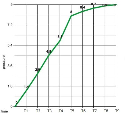
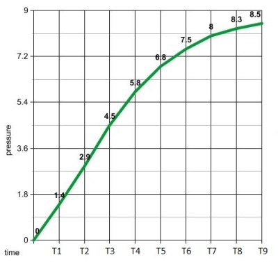
We can use a similar process with our pressure measurements to distinguish between a gas and a liquid. The rate of change units for this process is PSI per second. We need to calculate this rate as the liquid is being added. If it gets too high, we know gas has entered the container. First, we need some data to work with. Let us make two controls. One will give us the pressure data for a normal liquid add, as seen in the graph above and to the left. The other is the pressure data when the liquid runs out, shown in the graph on the right. Visually, it’s easy to see when gas gets in the system. We see a surge between time’s T4 and T5. If we calculate the average rate of change between 1 second time intervals, we see that all but one of them are less that 2 psi/sec. Between time’s 4 and 5 on the gas graph, the average rate of change is 2.2 psi/sec. The next highest change is 1.6 psi/sec between times T2 and T3.
So now we know what we need to do. Monitor the rates of change and error out when it gets above 2 psi/sec.
Our psuedo code would look something like:
pressure = x;
delay(1000);
pressure = y
rateOfChange = (y - x);
if (rateOfChange > 2)
digitalWrite(13, HIGH);  //stop machine and sound alarm
Instantaneous Rate of Change
It appears that looking at the average rate of change over a 1 second time interval is all we need to solve our problem. If we wanted to get an instantaneous rate of change at a specific time, we need to make that 1 second time interval smaller. Let us remember that our microcontroller is much faster than the changing pressure data. This gives us the ability to calculate an average rate of change over very small time intervals. If we make them small enough, the average rate of change and instantaneous rate of change are essentially the same.
Therefore, all we need to do to get our derivative is make the delay smaller, say 50ms. You can’t make it too small, or your rate of change will be zero. The delay value would need to be tailored to the specific machine by some old fashioned trial and error.
Taking the Limit in a Microcontroller?
One thing we have not touched on is the idea of the limit within a microcontroller. Mainly, because we don’t need it. Going back to our car example, if we can calculate the average speed of the car between mile marker one and mile marker 0.0001, why do we need to go though a limiting process? We already have our instantaneous rate of change with the single calculation.
One can argue that the idea behind the derivative is to converge on a single number while going though a limiting process. Is it possible to do this with incoming data of no known function? Let’s try, shall we? We can take advantage of the large gap between the incoming data’s rate of change and the processor’s speed to formulate a plan.
Let’s revisit our original problem and set up an array. We’ll fill the array with pressure data every 10ms. We wait 2 seconds and obtain 200 data points. Our goal is to get the instantaneous rate of change of the middle data point by taking a limit and converging on a single number.
We start by calculating the average rate of change between data points 200 and 150. We save the value to a variable. We then get the rate of change between points 150 and 125. We then compare our result to our previous rate by taking the difference. We continue this process of getting the rate of change between increasingly smaller amounts of time and comparing them by taking the difference. When the difference is a very small number, we know we have converged on a single value.
We then repeat the process in the opposite direction. We calculate the average rate of change between data points 0 and 50. Then 50 and 75. We continue the process just as before until we converge on a single number.
If our idea works, we’ll come up with two values that would look something like 1.3999 and 1.4001 We say our instantaneous rate of change at T1 is 1.4 psi per second. Then we just keep repeating this process.
Now it’s your turn. Think you have the chops to code this limiting process?
Filed under: Arduino Hacks, Hackaday Columns


