Planet Arduino

Today’s makers have access to the most advanced materials, resources, and support in history, and it’s improving all the time. The downside is that finding the right software can sometimes feel confusing and overwhelming. There are seemingly endless options, all with different attributes and advantages.

In this article, we’re here to help make things easier. We’ll walk you through the best software for makers at each experience level — beginner, intermediate, and expert — and help you identify the right software for your needs.

The best maker software for each experience level

Beginner-level software

If you’re new to the world of making, you’ll likely have some specific needs and requirements that won’t apply to more experienced folks.

For example, you’ll want software that’s forgiving and beginner-friendly, that comes with more opportunities to learn the basics, and is easy enough that you won’t be discouraged from making.

With that in mind, here are our top picks for the best beginner-level maker software.

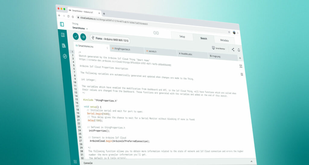
Arduino IDE

Arduino is one of the most well-established and well-known platforms for makers of all levels. Arduino’s microcontrollers allow you to program projects with your own custom code, creating gadgets that work exactly the way you want them to.

If you’re new to the game, you’ll want to start with a microcontroller that’s suitable for beginners. The Arduino IDE is perfect for this: it’s free, user-friendly, and leverages a simplified version of the C/C++ programming languages so you can learn the basics in a fun and rewarding way.

TinkerCAD

Since it first came onto the scene in 2011, TinkerCAD has been a great choice for beginners looking to get started with making their own projects.

As a CAD (computer-aided design) software, TinkerCAD is a fantastic tool for designers and can be used to create models for 3D printing. 

Due to its beginner-friendly nature, TinkerCAD is often used in schools to help learners get to grips with basic coding and design, building their own elementary tech projects. It’s also completely free of charge.

The advantage of using TinkerCAD is that it also contains a simple circuit designer and visual code tool useful to generate the code for Arduino boards.

Intermediate-level software 

Once you’ve learned the basics of making, you’ll likely be craving some more challenging and stimulating projects.

Taking your coding skills to the next level requires more sophisticated software, allowing you to be more adventurous and ambitious with your plans. The good news is that there is plenty of software out there for intermediate makers. Let’s take a look at some examples.

Python

Python is one of the most well-known programming languages out there, and it’s compatible with most maker-friendly platforms and microcontrollers.

Python works well with Arduino hardware, and is especially well-suited for projects that use sensors and other components. You don’t need to be a coding wizard to start using Python in this way, but you will need some familiarity and experience.

Check out this project — a Nicla Vision-based fire detector built by Arduino user Shakhizat Nurgaliyev using Python. Shakhizat created an entirely generated dataset and then trained a model on that data to detect fires.

MicroPython

MicroPython is an experimental, lean, and lightweight implementation of the programming language Python, and it’s designed specifically to be used with microcontrollers.

This makes it ideal for use with Arduino projects, and it works especially well with those that use sensors and similar components. MicroPython does require a base of coding knowledge to use, but you don’t need to be an expert.

Visual Studio Code

Visual Studio Code, often abbreviated as VS Code, is an open-source editor created by Microsoft that is compatible with Windows, Linux, and macOS. 

It offers a range of features such as debugging support, syntax highlighting, smart code completion, snippets, code refactoring, and integrated Git functionality. Visual Studio Code can be used to develop code for Arduino boards, and, by using the available extensions, you can upload code directly to the Arduino boards.

Node-RED

Node-RED is built to bring hardware devices, software, and online services together, creating ever more interesting and advanced projects.

It works especially well with IoT projects — and is a great choice if you want to integrate platforms like Arduino with other devices to build your own custom designs for use in your home.

Node-RED’s browser-based editor and built-in library make it a powerful tool for those with some coding experience to make new projects.

Arduino’s Portenta X8 can host a Node-RED instance running it on a container, making it easy to connect and integrate several different services, either locally or online with Arduino Cloud or third-party software. 

In this project, David Beamonte used Node-RED and Arduino Cloud, to integrate a TP-Link smart Wi-Fi plug with other projects. This way, they were able to link multiple smart home devices together and control them from one central hub.

Expert-level software

Are you a true veteran of making and coding? Fluent in more programming languages than you can remember, with a host of impressive projects under your belt and a slot at next year’s Maker Faire?

If so, you have the skills to achieve some truly exciting things. Let’s take a look at the software available for expert-level makers.

MATLAB

MATLAB is an advanced piece of software that works well with Arduino hardware and similar products. 

It’s especially useful when building projects that require data analysis and complex, large-scale computations. Proficiency in MATLAB can lead to some truly impressive creations, but it takes a solid amount of experience and skill to realize those results.

Arduino users MadhuGovindarajan and ssalunkhe used MATLAB to build their very own lane-following rover. The project used the rover from Arduino’s Engineering Kit, combined with an algorithm that allows the rover to stay within a designated lane while driving.

The Arduino Engineering kit contains three different projects that involve physical hardware and MATLAB/Simulink to create amazing results. 

C/C++ IDEs

The programming languages C and C++ have been around for decades, underpinning the worlds of computer science and software engineering.

If you have a solid base of coding ability, you can use C/C++ development environments to program Arduino boards and create ever more advanced and impressive projects.

Other resources

GitHub

Do you want to share your code with your mates, or with the world? 

If so, GitHub is the perfect place to do it. It’s an open-source community with multiple contributors and lots of integrations with developer-oriented software. 

Inside, you’ll find more than 300 million projects, known as repos. Makers use the platform to share their work, but it can also be useful to take a look and draw inspiration from the trending repositories.

AI/ML

AI is making headlines all over the world, but it extends far beyond ChatGPT.

Makers today have access to a wealth of fantastic tools to speed up work, correct errors, and document your shiny new code. Check out GitHub copilot and OpenAI Codex to get started.

Using software with Arduino

By combining the right software tools with Arduino’s products, you have the perfect recipe for your next awesome project.

If you want to gain inspiration, or share your own work with our community, check out the Arduino Project Hub where you can search for projects and filter by type and difficulty level.

The post The best maker software by experience level appeared first on Arduino Blog.

The Arduino development scene just got a big upgrade with the introduction of the Arduino Cloud...

The post Revolutionizing Arduino Development: Exploring the Power and Potential of the Arduino Cloud Editor appeared first on Electronics-Lab.com.

I was intrigued by a recent project I saw that used two LED matrices placed diagonally to create an hourglass. The animated movement of the LEDs seemed a good simulation of the sand particles moving through the hourglass.

As is common, the project emphasized on how the hardware was wired together, which is trivial, without much explanation of its more challenging/interesting software aspects.

Additionally, most of the solutions I saw used an inertial position sensor to determine the position of the matrix, which seemed overkill for the simple functionality required.

So I decided to explore this topic and here is my solution.

Hourglass Basics

An hourglass (also known as a sand clock) is used to measure the passage of time. An hourglass is usually made up of two symmetric glass bulbs connected vertically by a narrow neck through which sand, or other suitable material, goes from the upper to the lower bulb under the action of gravity. The hourglass is turned upside-down to start another timer when all the sand runs into the bottom bulb.

Each hourglass is designed to measure a specific time interval – the time it takes to empty one bulb into the other. This time is regulated by factors that include the amount and size of the sand particles, the bulb size and the neck width.

Hardware Assembly

LED Matrices

The LED matrices are the commonly available 8×8 LED modules controlled by a MAX7219 controller. For this project the matrices with smaller PCBs that fit under the LED module are the best form factor.

Orientation Sensor

To keep things simple the orientation of the matrix is measured by a simple digital input wired to a tilt switch. These small and inexpensive sensors are available in many shapes and sizes, but all work similarly – a digital signal in one orientation and no signal for the opposite orientation, as shown in the figure below.

Internally the switch commonly has a metal ball that moves to make/break the electrical circuit.

This sensor is not able to detect intermediate states (eg, the hourglass on its side) but I am happy to live with that tradeoff compared to a much more expensive inertial sensor.

Hourglass Bezel

For testing purposes, using Fusion 360, I designed and 3D printed an hourglass shaped bezel to hold the 2 modules a jam fit.

This keeps the modules in the correct diagonal orientation with respect to each other and allows me to conveniently rotate the whole device easily.

Software Implementation

The software discussed in this section is available as the MD_MAX72xx_Hourglass example code with the MD_MAX72xx library.

Simulating the Hourglass

When thinking about this closed system, the top bulb can be considered a silo filled with sand with an exit at the bottom. As the sand passes through the neck, the sand particles above the moved particle also move into the void below and this is repeated all the way to the top of the sand reservoir.

As the mechanism is driven by gravity, it can be thought of as the particles trying to minimize their potential energy with respect to the hourglass neck.

Once the sand passes the neck it will fall (again trying to minimize the potential energy with respect to the base of the lower bulb) until it reaches the rest of the sand pile, at which time it will move over the surface of the existing pile trying to find its minimum energy state.

A good proxy for simulating the energy of each particle could be the distance between each particle and the neck/base, as potential energy is related to the height of each particle from the relevant ‘zero energy’ point.

Some Definitions

As these ‘zero energy’ point are points to which the particles are attracted, I decided to call them attractors in the software.

There are four attractors relevant to the simulation, shown in the figure at left, called HIHI, HI, LO, LOLO. When particles are travelling from the top to the bottom bulb, they are initially attracted to the HI attractor (the bottom of the top bulb) and then the LOLO attractor when they pass through the neck.

Conversely when the hourglass is turned over the attractors become the LO and HIHI attractors.

When wiring the matrices together, the module with the HI and HIHI attractor is module 0 (the first in the chain) and the other is module 1. The electrical connections are from the top to the bottom modules, as shown on the left.

Software Structure

There is a relatively simple structure to this software:

1. Initialization (ie, the setup() function).
2. Check if hourglass has changed orientation.
3. At the appropriate time
   • Moving all the particles in both bulbs
   • Moving a particle from the upper to the lower bulb if one is ready to drop
   • Updating the matrices with the new arrangement

We’ll discuss each of these in turn below.

Data Structures and Static Data

Two simple data structures are defined to help manage the simulation.

The first is small container for the row and column coordinates of a LED ‘particle’.

typedef struct
{
  int8_t r, c;
} coord_t;

The next is the definition of a particle, which comprises its coordinates on the display and the attractor that is controlling its motion.

typedef struct
{
  attractorId_t att;
  coord_t p;
} particle_t;

The attractor enumerated type has the values as discussed earlier. The enumerated values are specifically nominated as they are used as the index into an array of constant coordinates for each of the attractors.

typedef enum 
{ 
  ATT_HIHI = 0,
  ATT_HI = 1,
  ATT_LO = 2,
  ATT_LOLO = 3
} attractorId_t;

Finally, an enumerated type is defined to track the current orientation of the hourglass (ie, the direction in which the particles are flowing due to the action of gravity).

// flow direction for particles (HI->LO or LO->HI)
typedef enum 
{ 
  FLOW_HI2LO, 
  FLOW_LO2HI 
} flowDirection_t;

Initialization

The particle array is statically initialized when it is declared. As the matrix is on the diagonal corner, this seemed an easier way to get a specific pattern in the top bulb at the start.

The normal hardware initialization happens in setup(), and the display is updated with the starting particle arrangement.

Check Hourglass Orientation

The hourglass orientation is given by a simple digital input from the tilt sensor. When that input changes it needs to be processed into a direction indicator (FLOW_* enumerated value) and a different attractor (ATT_*) for each particle.

For example, if a particle is in the top bulb, travelling FLOW_HI2LO directions, is currently attracted to ATT_HI. Once the flow is reversed (to FLOW_LO2HI) that particle is now attracted to HIHI.

Moving Particles

Particle moves occur periodically, controlled by the total timer duration, 30 seconds for the example code. Given that all the particles need to transition to the next bulb by the end of the period, each time slice is a total time divided by the number of particles.

For each particle, each of the 8 points surrounding the particle need to be tested to see if the particle should move into that location. A particle can move into a new location if:

1. The location is unoccupied.
2. The location is within the bounds of the hourglass bulb containing the particle.
3. The distance to the particle’s attractor is the minimum distance of the current set of potential locations.

The distance between the particle and its attractor is the length of the line segment that connects the two points, given by d=√((r2 – r1)² + (c2 – c1)²). As d is just for comparison the square root is unnecessary and the software uses d².

If two or more points are found to be equal minima, then a random choice is made between them.

Transition Particles

Once all the particles have moved, a special check is made to see if a particle is at the ATT_HI or ATT_LO points (depending on the flow direction).

If one is found, it is moved to the top of the lower bulb if there is no other particle there and its attractor is changed so that it travels to the bottom of the hourglass.

Display Update

The display update clears the display and then redraws all the particles at their current coordinates.

So does it work?

Given the simplicity of the approach and simulation code, the LED hourglass display looks good and works surprisingly well.

In the first part we looked at the HX711 hardware for implementing weigh scales systems.

This part will cover how software interacts with the hardware, requirements for a library and how to write a weigh scale application.

All the code described in this article can be found in my libraries code repository as the MD_HX711 library and examples.

Requirements

The most basic components of weighing machines a weight sensor, processing device and an interface (for example, these could be a load cell/HX711, a microprocessor and a display, respectively). They usually also have a method for taring the weight (eg, a switch). Other advanced features can be built into the device but they are refinements on the basics.

The simplest user interface for the scale is to continuously send to the interface the measured value. For a display output this would be just shown (like bathroom or kitchen scales) and/or it could be output through an external interface such as a serial port. Many industrial weight scales work exactly like this.

Therefore to implement a minimal weighing system we need a software framework, such as an Arduino library, that:

1. Enables access to all the HX711 features (ie, both channels of data, resetting the device and Channel A gain selection).
2. Can work in the background so that the application code implementing the weight scale functionality is free from dealing with hardware related operations. Preferably this works by either periodically polling the HX711 or by external interrupt.
3. Allows the device to be tared and calibrated.
4. As a minimum provides the readings from the device as raw, tared or calibrated values.

There are many HX711 libraries available and many provide lots of functions above the basics outlined above. However, I could not find one allowed easy access to Channel B or worked using an external interrupt. So I decided that it was time to write my own.

Library Implementation

Reading Device Data

The core of the library is a function used to implement the device communication protocol described in the previous post. The HX711ReadData() code is a straightforward sequential implementation of the CLK/DAT sequencing and timing required by the interface. The function returns the 24-bit DAC number received as a 32-bit integer.

int32_t MD_HX711::HX711ReadData(uint8_t mode)
// read data and set the mode for next read depending on what 
// options are selected in the library
{
  // local variables are faster for pins
  uint8_t clk = _pinClk;
  uint8_t data = _pinDat;

  // data read controls
  int32_t value = 0;
  uint32_t mask = 0x800000L;
    
  do   // Read data bits from the HX711
  {
    digitalWrite(clk, HIGH);

    delayMicroseconds(1);   // T2 typ 1us

    if (digitalRead(data) == HIGH) value |= mask;
    digitalWrite(clk, LOW); 

    delayMicroseconds(1);  // T3 typ 1us
    mask >>= 1;
  } while (mask > 0);

  // Set the mode for the next read (just keep clocking)
  do
  {
    digitalWrite(clk, HIGH);
    delayMicroseconds(1);
    digitalWrite(clk, LOW);
    delayMicroseconds(1);
    mode--;
  } while (mode > 0);

  return(value);
}

Note that the microsecond timing in this function is moot given that digitalWrite() and digitalRead() are quite slow compared to native processor register read/write.

HX711ReadData() is called from readNB() (read non-blocking), which puts the correct library context around the hardware call. This includes:

• working out which channel we need to ask for in the next iteration.
• setting the gain for the channel being requested.
• managing the interrupt context.
• saving the data received to the correct internal storage register.

The reason that we have a non-blocking read is that this method is designed to be called safely by an ISR for an external interrupt.

void MD_HX711::readNB(void)
// NON-Blocking read the data from the HX711 in an IRQ 
// safe manner.
{
  uint8_t extras = 0;
  int32_t value;

  _inISR = true;

  // set the next read channel
  if (_enableB) _nextReadA = !_nextReadA;

  // now work out how many extra clock cycles send when reading data
  if (!_nextReadA)            extras = 2; // Channel B gain 32
  else if (_mode == GAIN_128) extras = 1; // Channel A gain 128
  else                        extras = 3; // Channel B gain 64

  // do the read
  noInterrupts();
  value = HX711ReadData(extras);
  interrupts();

  // sign extend the returned data
  if (value & 0x800000) value |= 0xff000000;

  // save the data to the right index value
  channel_t ch = (_enableB && _nextReadA) ? CH_B : CH_A;
  _chanData[ch].raw = value;

  // increment the counter
  _readCounter++;

  _inISR = false;
}

The last received data for each channel is stored in library registers and can be retrieved using the getRaw(), getTared() and getCalibrated() methods, depending on what data the application needs.

Device Reset

The HX711 is reset by powering it down using the CLK pin held HIGH then back up again a very small time later.

inline void MD_HX711::powerDown(void)
// Set the CLK to low for at least 60us.
{
  digitalWrite(_pinClk, HIGH);
  delayMicroseconds(64);   // at least 60us HIGH
}

inline void MD_HX711::powerUp(void)
// set the CLK to high
{
  digitalWrite(_pinClk, LOW);
}

This resets the device into a default state, so the library implements a reset() method that does the same and keeps the library and device synchronized.

void MD_HX711::reset(void)
// set defaults and power cycle the hardware
{
  powerDown();
  powerUp();

  // set the library defaults
  enableChannelB(false);
  setGainA(GAIN_128);
  disableISR();
  _nextReadA = true;
  _readCounter = 0;
  for (uint8_t ch = 0; ch < NUM_CHAN; ch++)
  {
    _chanData[ch].raw = 0;
    _chanData[ch].tare = 0;
    _chanData[ch].calib = 0;
    _chanData[ch].range = 0.0;
  }
}

Tare and Calibration

The values returned from the hardware are 24-bit ADC values converting the amplified Wheatstone differential voltage to a number. This number must be calibrated to convert the value to a meaningful reading.

To calibrate the readings we first need to assume the Wheatstone bridge provides a linear response to the changes in weight (ie, there is a simple proportional relationship). This is the blue line in the figure. We know this assumption is not correct (see this article) but it is close enough if we choose the right load cell for the application.

The first part of calibration is to tare the readings with no force on the sensor (autoZeroTare() or setTare() methods). This provides the information to shift the ‘raw’ blue response curve to the green curve (line A₀B₀ shift to A₁B₁) by subtracting the tare ADC value. This locks in the zero point for the conversions and returned by the getTared() method.

The next part is to calibrate the actual slope of the conversion line – moving the green curve A₁B₁ to the red curve A₁B₂ in the diagram. This is done by applying a known force to the sensor (such as a known mass) and noting the ADC value returned (setCalibration()).

By setting the zero point and one known point, and assuming a linear response in the range of values being measured, the converted value y can be easily computed for any ADC value x using the getCalibrated() method.

Polled or External Interrupt?

The library supports both a polled and an interrupt driven approach to obtaining data from the HX711. Up to four separate HX711 devices on unique external interrupts are supported, using the technique described in this past post.

The enableInterruptMode() method is used by the application to toggle interrupt mode on/off as needed.

Polled Mode

This is the default operating mode for the library.

In polled mode the public read() method is synchronously invoked to wait for and obtain the next value from the hardware. If channel B is enabled the library will alternate reading channels (A, B, A, B, etc). The read() method returns the identifier of the channel last processed and the data is retrieved with getRaw(), getTared() and getCalibrated(), as required.

As the read() method is synchronous (it blocks waiting for the next data to be available read from the hardware) the isReady() method can be used to determine if there is data ready for processing. This allows an application to check before calling read() to avoid unnecessary application delays caused by the library.

Interrupt Mode

In interrupt mode the library will process data received from the HX711 in the background, based on an interrupt generated by the device DAT signal going low.

Interrupt mode requires that the I/O pin connected to the DAT signal supports external interrupts (eg, for an Arduino Uno this would be pins 2 or 3).

The application can monitor the getReadCount() method to determine when new data has been received. In interrupt mode the read() method becomes non-blocking and returns the id of the channel whose data was the last received so that it can be read with getRaw(), getTared() and getCalibrated().

Prototyping Weigh Scales

Once the basic hardware related functions of the library were coded and broadly tested, it was time to prototype a weight scale to complete the weigh scale code.

Hardware

I was testing with a 1kg bar-type load cell, so a small scale was adequate. A 100mm diameter top and a bottom plate were modelled in Fusion360, shown below, and 3D printed in ABS.

The top plate is a solid disc. The bottom is more open to save material and give access to the screws for joining the top plate and load cell. Both plates include a small pad to lift the load cell so that it is cantilevered it between the two plates. Machine screws (M4) connect all the components together.

Additional hardware required for this prototype was:

• A 2 line by 20 character LCD module. In this instance it used an I²C interface to the processor, but any other size module and interface that works with LiquidCrystal (or clones) library will work.
• A tact switch to tare and calibrate the scale.

The final configuration is shown in the photo above, along with a few of the objects used to test the scale and my 1kg bag of rice used to for calibration.

Software

As the library does most of the heavy lifting, the application software becomes straighforward.

The software described here is the MD_HX711_WeighScale example from the library.

This example implements a weigh scale that

• Can be tared and calibrated using a tact single switch. A Single press of the switch sets the tare, double press sets the calibration to 1000g.
• Tare and calibration settings are stored in EEPROM and loaded at startup.
• Updates the LCD display with the current weight as soon as a new weight is available.
• Demonstrates receiving data from the HX711 in either polled or interrupt driven mode, set by a #define at compile time.

Configuration Parameters are loaded at startup. The EEPROM data includes two signature bytes so that the software can detect a ‘first time’ run and initialize the data to sensible defaults. All changes to configuration values are immediately and transparently saved to EEPROM.

The tact switch is managed by the MD_UISwitch library (also described in this previous post). This allows the application to test for either a press/double press in the main loop() and do the necessary for each case.

Taring is done to set the scale ‘zero’ by a simple pressing of the tact switch. This is usually when the sale is empty by could equally be when the scale has a container on it.

Calibration is carried out by putting a known 1000g weight (my not-very-accurate bag of rice) on the scale and double pressing the switch.

This application needs to be non-blocking for the user switch to work properly. In this case it turns out there is minimal difference to the application’s structure between interrupt and polled modes. In polled mode it monitors isReady() before calling read() to read the data; in interrupt mode it checks getReadCount() to know when new data is available.

One wrinkle is that when the weight is zero, ADC noise fluctuation around the zero point causes the scale to display 0.0 and -0.0. To prevent what looks like a flickering minus sign, the application calculates and displays a ‘damped’ weight calculated as

float dampedWeight(float newReading)
// Dampen the fluctuations in readings value and make any small // negative values 0.0
{
  const float PORTION = 0.80;
  static float lastReading = 0.0;

  // dampen
  lastReading += PORTION * (newReading - lastReading);

  // kill small negative values
  if (lastReading < 0.0 && lastReading > -0.1)
    lastReading = 0.0;

  return(lastReading);
}

If a weight is negative by less that the least significant figure (ie between 0.0 and -0.1) then we can display it as zero. This completely eliminates the visual distraction of the ‘flickering’ minus.

Additionally, this function also dampens the changes to the displayed weight by only adding in PORTION (80%) of the change between the current and last reading. This dampens the ADC noise but also has the side effect of a pleasing ‘converging value’ animation on the weighscale display.

If you search for ‘Arduino’ and ‘weighing’ you very quickly come across the HX711 board module and an associated world of strain gauges and load cells.

All this looked interesting with some learning along the way. The result is that I took a dive into the subject and ended up with some new knowledge and ideas for the future.

In this first part I cover the hardware requirements and in the next how to write software to implement a weighing system.

The HX711 ADC

The HX711 is a precision 24-bit Analog to Digital Converter (ADC) designed for weigh scales and industrial control applications. It readily obtainable from all the usual online marketplaces as ready-made modules implementing the standard datasheet circuit.

The IC interfaces directly with a up to two Wheatstone Bridge load cell’s differential outputs and incorporate signal amplifiers.

Channel A differential input can be programmed with a gain of 128 or 64. Channel B has a fixed gain of 32.

Large gains are needed to accommodate the small output signal from the sensor. When a 5V supply is used for the sensor, the gain corresponds to a full-scale differential input voltage of ±20mV with gain 128, ±40mV for 64 and ±80mV for 32.

Load Cells

Load cells come in various shapes and are rated from 0.1kg to over 1000kg full scale. They come in many different types of form factors but the two most common are bar and strain gauge types.

Bar-type Load Cells

Bar type load cells are straight bars with strain gauges attached to the point where it has maximum bending. A variant of straight bar is the S type cell design for tension (pulling) applications.

Each load cell has four strain gauges connected in a Wheatstone Bridge formation. The labeled colors correspond to the color-coding convention coding of load cells. Red, black, green and white wires are connected to the load cell’s strain gauge and yellow is an optional ground or shield wire to lessen EMI.

The direction of the force arrow labels on the load cells must match the direction of resultant force. If the resultant force is straight down (the usual in a weighing application) then the load cells must be installed so with the force arrow labels pointing down.

Strain Gauge Load Cells

Strain gauge load cells are commonly seen on the corners of bathroom scales and similar ‘platform’ type applications. Each load cell is a half Wheatstone bridge, as shown below.

This type of load cell must be combined into a circuit of 2 or 4 gauges to create the full Wheatstone bridge, with each side of the bridge including the strain resistors from two of the strain gauge load cells. The circuit for combining four strain gauges is illustrated below.

A simple way to combine the wiring is to create a Combinator Board. Here the wires from the individual strain gauge cells are joined in a hub arrangement, producing the required Wheatstone Bridge connections. Shown below is the hub connection for a four sensor configuration.

Module Wire Connections

The HX711 module’s A channel interfaces to the load cell through four wires labeled E+ (or RED), E- (BLK), A-(WHT), A+(GRN), and an optional shielding ground SD(YLW) on the circuit board.

The B Channel interfaces to a separate load cell through the E+, E- (common with Channel A) and B+, B- connections on the circuit board.

E+ and E- are the positive voltage and ground connections to load cell; the A+/A-, B+/B- the differential outputs from the load cell.

The module is connected to the processor’s power supply (Vcc and GND) and 2 additional processor digital input pins to the module’s DAT (or DT) and CLK (or SCK). These digital pins are used to manage the limited configuration options available and read the data from the HX711.

Hardware Control

Sampling Rate

The HX711 can sample at 10 samples per second (SPS or Hz) or 80Hz, set by the RATE pin on the IC.

Some module boards have a jumper on the reverse side of the board to set the rate, as shown below. Connecting RATE to 1 (Vcc) sets 80Hz and 0 (GND) is 10Hz.

Data Read and Gain Control

CLK is set by the processor, DAT is read by the processor. These two
digital signals make up the serial interface to the HX711.

CLK should be kept LOW by the processor unless clocking during a read cycle.

The data is read as 24 bits clocked out, one bit per clock cycle, from the HX711. Additional clock transitions (+1 to +3) are used to set the mode for the next read cycle according to the handshaking sequence below.

• When an ADC reading is not available, DAT is set HIGH by the HX711. CLK is held LOW by the processor.
• When DAT goes to LOW, the next ADC conversion can be read by the processor.
• The processor sends 25 to 27 positive (transition LOW to HIGH) CLK pulses to shift the data out through DAT one bit per clock pulse, starting with the most significant bit (MSB), until all 24 data bits are shifted out.
• The HX711 will then hold DAT HIGH for the remainder of the clock pulses.
• Channel and Gain selection for the next read is controlled by the number of additional CLK pulses (+1 to +3) send to the HX711, for a total of 25 to 27 clock pulses as shown in the table below.

Fewer than 25 and more than 27 clock pulses in one communication cycle will cause a serial communication error requiring a HX711 reset.

Reset and Power Down Sequence

When power is first applied, the power-on circuitry will reset the IC.

The CLK output from the processor is also used to reset the HX711 IC.

When CLK is

• LOW, the HX711 is in normal working mode.
• changed from LOW to HIGH and stays HIGH for longer than 60μs, the HX711 is powered down. It remains in this state while the signal remains high.
• changed from HIGH to LOW, the HX711 resets and restarts normal working mode.

Following a reset the hardware defaults to Channel A input, gain 128.

In Part 2 we’ll look at the software for this module and how to use the hardware/software to implement a weigh scale system.

If you search for ‘Arduino’ and ‘weighing’ you very quickly come across the HX711 board module and an associated world of strain gauges and load cells.

All this looked interesting with some learning along the way. The result is that I took a dive into the subject and ended up with some new knowledge and ideas for the future.

In this first part I cover the hardware requirements and in the next how to write software to implement a weighing system.

The HX711 ADC

The HX711 is a precision 24-bit Analog to Digital Converter (ADC) designed for weigh scales and industrial control applications. It readily obtainable from all the usual online marketplaces as ready-made modules implementing the standard datasheet circuit.

The IC interfaces directly with a up to two Wheatstone Bridge load cell’s differential outputs and incorporate signal amplifiers.

Channel A differential input can be programmed with a gain of 128 or 64. Channel B has a fixed gain of 32.

Large gains are needed to accommodate the small output signal from the sensor. When a 5V supply is used for the sensor, the gain corresponds to a full-scale differential input voltage of ±20mV with gain 128, ±40mV for 64 and ±80mV for 32.

Load Cells

Load cells come in various shapes and are rated from 0.1kg to over 1000kg full scale. They come in many different types of form factors but the two most common are bar and strain gauge types.

Bar-type Load Cells

Bar type load cells are straight bars with strain gauges attached to the point where it has maximum bending. A variant of straight bar is the S type cell design for tension (pulling) applications.

Each load cell has four strain gauges connected in a Wheatstone Bridge formation. The labeled colors correspond to the color-coding convention coding of load cells. Red, black, green and white wires are connected to the load cell’s strain gauge and yellow is an optional ground or shield wire to lessen EMI.

The direction of the force arrow labels on the load cells must match the direction of resultant force. If the resultant force is straight down (the usual in a weighing application) then the load cells must be installed so with the force arrow labels pointing down.

Strain Gauge Load Cells

Strain gauge load cells are commonly seen on the corners of bathroom scales and similar ‘platform’ type applications. Each load cell is a half Wheatstone bridge, as shown below.

This type of load cell must be combined into a circuit of 2 or 4 gauges to create the full Wheatstone bridge, with each side of the bridge including the strain resistors from two of the strain gauge load cells. The circuit for combining four strain gauges is illustrated below.

A simple way to combine the wiring is to create a Combinator Board. Here the wires from the individual strain gauge cells are joined in a hub arrangement, producing the required Wheatstone Bridge connections. Shown below is the hub connection for a four sensor configuration.

Module Wire Connections

The HX711 module’s A channel interfaces to the load cell through four wires labeled E+ (or RED), E- (BLK), A-(WHT), A+(GRN), and an optional shielding ground SD(YLW) on the circuit board.

The B Channel interfaces to a separate load cell through the E+, E- (common with Channel A) and B+, B- connections on the circuit board.

E+ and E- are the positive voltage and ground connections to load cell; the A+/A-, B+/B- the differential outputs from the load cell.

The module is connected to the processor’s power supply (Vcc and GND) and 2 additional processor digital input pins to the module’s DAT (or DT) and CLK (or SCK). These digital pins are used to manage the limited configuration options available and read the data from the HX711.

Hardware Control

Sampling Rate

The HX711 can sample at 10 samples per second (SPS or Hz) or 80Hz, set by the RATE pin on the IC.

Some module boards have a jumper on the reverse side of the board to set the rate, as shown below. Connecting RATE to 1 (Vcc) sets 80Hz and 0 (GND) is 10Hz.

Data Read and Gain Control

CLK is set by the processor, DAT is read by the processor. These two
digital signals make up the serial interface to the HX711.

CLK should be kept LOW by the processor unless clocking during a read cycle.

The data is read as 24 bits clocked out, one bit per clock cycle, from the HX711. Additional clock transitions (+1 to +3) are used to set the mode for the next read cycle according to the handshaking sequence below.

• When an ADC reading is not available, DAT is set HIGH by the HX711. CLK is held LOW by the processor.
• When DAT goes to LOW, the next ADC conversion can be read by the processor.
• The processor sends 25 to 27 positive (transition LOW to HIGH) CLK pulses to shift the data out through DAT one bit per clock pulse, starting with the most significant bit (MSB), until all 24 data bits are shifted out.
• The HX711 will then hold DAT HIGH for the remainder of the clock pulses.
• Channel and Gain selection for the next read is controlled by the number of additional CLK pulses (+1 to +3) send to the HX711, for a total of 25 to 27 clock pulses as shown in the table below.

Fewer than 25 and more than 27 clock pulses in one communication cycle will cause a serial communication error requiring a HX711 reset.

Reset and Power Down Sequence

When power is first applied, the power-on circuitry will reset the IC.

The CLK output from the processor is also used to reset the HX711 IC.

When CLK is

• LOW, the HX711 is in normal working mode.
• changed from LOW to HIGH and stays HIGH for longer than 60μs, the HX711 is powered down. It remains in this state while the signal remains high.
• changed from HIGH to LOW, the HX711 resets and restarts normal working mode.

Following a reset the hardware defaults to Channel A input, gain 128.

In Part 2 we’ll look at the software for this module and how to use the hardware/software to implement a weigh scale system.

Scoreboards seem to be quite popular as beginner projects but the results are often very specific to the hardware used and very ‘hard coded’ to the original purpose.

It seemed to me that there are some parts of this style of application that are generic and probably independent to the type of scoreboard (sport and/or hardware used). I wanted to explore which parts and how this could drive a generic framework to create and update any scoreboard.

Scoreboard basics

A scoreboard is a large board, for example at a sports ground or stadium, on which the score in a game or match is displayed for the audience and participants. This display is typically square or rectangular in shape and contains all of the information relevant the sport/game such as home and guest score, game elapsed time, quarter/half indicator, other clock information, etc.

A good scoreboard is simple – it should be easy to read and quick to understand. It should contain clear information specific to the game being played and may include important game metrics. These metrics can greatly complicate the layout and size of displays for some sports – in my experience Cricket is an extreme example (shown below).

So what’s generic about this?

For simplicity I’ll just consider a sports scoreboard similar to the type shown below.

Analyzing the data displayed by this style of scoreboard, we can see a limited range of types of information:

• Numeric Fields. By far the majority of information on a scoreboard consists of numeric fields.
• Clocks. There is usually at least one game clock (duration or countdown) and often a second clock (eg, a shot clock in basketball).
• Static Elements. These are labels (Home, Guest, Score, etc) and separation lines that don’t change during the course of the game. These invariant elements are often built into the physical construction of the scoreboard.
  Some labels may be static just for one match (player names, team names) and these are often handled using replaceable signs or as text fields on software driven displays.
• Graphical Elements. Some data elements may be represented in graphical form such as dots, lines or icons. The underlying data is usually numeric (for example true/false or a count).

Building a framework

The framework described here is included in the scoreboard examples (the file scoreboard.h in MD_MAXPanel_SB_*) accompanying the MD_MAXPanel library. While the current framework uses a 40×32 LED panel as the scoreboard, it should be straightforward to change for alternative output hardware.

Defining the Scoreboard

For me, a useful framework takes the display and clock management functions away from the application and allows it concentrate on the functionality required for the scoreboard operator.

So, as a starting point, this means that all display field management will happen within the framework code (a C++ class in this implementation). Fields in this class are represented as a linked list of field attributes created by the application when defining the scoreboard. Each entry in the list is given a unique application defined numeric identifier id by the application.

  enum fieldType_t
  {
    NUMBER,   ///< a simple number
    MMMSS,    ///< time MMM:SS displayed
    MMSS,     ///< time MM:SS displayed
    SS        ///< time SS display only
  };

  struct field_t
  {
    uint8_t id;       ///< identifier
    fieldType_t type; ///< field type
    uint8_t x, y;     ///< field coordinates
    uint32_t value;   ///< current value of the field
    bool leadZero;    ///< field has leading zeroes
    uint8_t size;     ///< field size in characters/numbers
    field_t* next;    ///< next in the list
  };

The field has a coordinate x, y for its top left corner, a size (displayed characters), including the colon for time and leading zeroes if specified. The type of field determines how to interpret and display its current value. For clocks the current time is uniformly stored in seconds but can be displayed in the different formats specified.

A clock is a field that has associated with it additional information. A game clock will have a timeLimit it counts up to (or down from), a boolean status of whether it is stopped, and some in ternal management.

  struct clock_t
  {
    field_t* f;           ///< field associated with this timer
    uint32_t timeLimit;   ///< upper limit for time
    uint32_t timeLast;    ///< last time displayed/updated
    uint32_t timeToGo;    ///< time to go before next update
    bool countUp;         ///< counting up if true
    bool stopped;         ///< true if stopped
  };

To define a scoreboard an application needs to define the displayed fields (using fieldCreate()) and then associate a clock with those fields that are clocks (clockCreate()).

Managing Field Values

Fields only contain numeric values, so simple class methods to manage each field are fieldSetValue(), fieldGetValue() and fieldValueAdd() which do the obvious suggested by the method name.

Managing Clocks

For the clock fields the value is managed by the class rather than the application, although the field*() methods will still work correctly.

The clock value is incremented or decremented each second by the class. The application manipulates the status of a clock using

• clockStart() to stat the clock running.
• clockStop() to stop the clock running.
• clockToggle() to runs the clock if stopped and stops it if running.
• clockReset() to set the clock to the appropriate value depending on whether it is counting up or down.
• isClockRunning() to check its run status.

Display Updates

The application repeatedly calls the update() method to allow the class to run its management functions and update the display as required.

Updates are optimized to only change the display hardware when there has been a change to the scoreboard data. All changes occurring between after a call to update() are output at the next call to update().

Sample Applications

Simple scoreboard

The first application is a simple scoreboard showing 2 scores and a clock in MMSS format that counts up from zero time (example code MD_MAXPanel_SB_Simple).

The layout was planned using a spreadsheet to locate the fields and static elements of the display.

The prototype operator interface consists of a few tact switches managed by the MD_UISwitch library as follows:

• Clock Control – one switch to start and stop the clock. A long press resets the clock to zero.
• Score Up – one switch per score field to add +1 to the score.
• Score Down – One switch per score field to add -1 to the score. A long press resets the associated score to zero.

The final scoreboard is shown below. The static elements (lines) are drawn by the application during initialization.

Basketball scoreboard

To test the framework concepts further a more complex basketball scoreboard was created with 2 different clocks, more fields, more static elements and some graphical output (example code MD_MAXPanel_SB_BBall).

The display was planned on a spreadsheet, as before.

The operator interface consists of a few tact switches managed by the MD_UISwitch library as follows:

• Clock Control – one switch to start and stop the clock. A long press resets the clock to zero.
• Period Count Up – Increment the period counter. Once it reaches 4 it resets back to 0. The period is shown graphically as a sequence of 4 rectangles under the shot clock.
• Timeout Count Up – One switch per team to add +1 to the timeouts. Timeouts are reset to 0 once they reach 2. Timeouts are shown graphically as a line of 3 dots above the score.
• Score Up – One switch per score field to add +1 to the score.
• Score Down – One switch per score field to add -1 to the score. A long press resets the associated score to zero.
• Team Foul Up – One switch to increment the team foul count. Once this reaches 9 it resets to 0.
• Shot Clock Reset – One switch top reset the shot clock.
• Shot Clock Start/Stop – One switch to start and stop the shot clock.

Graphical elements are managed by the application as I could not find a ‘nice’ way to do this in the management class without creating excessive complexity in the class and how it is used.

The final scoreboard is shown below.

Conclusion

The results from this experiment are a bit of a mixed bag for me.

In simple applications, just showing scores and clocks, the framework works well and is a useful tool to simplify the management of the scoreboard.

However, if scoreboard graphical elements are included, I feel that the application still needs to do too much work outside of the management class, bringing it back into the ‘hard coded’ territory I was trying to avoid at the outset.

I may need to revisit this in future…

Scoreboards seem to be quite popular as beginner projects but the results are often very specific to the hardware used and very ‘hard coded’ to the original purpose.

It seemed to me that there are some parts of this style of application that are generic and probably independent to the type of scoreboard (sport and/or hardware used). I wanted to explore which parts and how this could drive a generic framework to create and update any scoreboard.

Scoreboard basics

A scoreboard is a large board, for example at a sports ground or stadium, on which the score in a game or match is displayed for the audience and participants. This display is typically square or rectangular in shape and contains all of the information relevant the sport/game such as home and guest score, game elapsed time, quarter/half indicator, other clock information, etc.

A good scoreboard is simple – it should be easy to read and quick to understand. It should contain clear information specific to the game being played and may include important game metrics. These metrics can greatly complicate the layout and size of displays for some sports – in my experience Cricket is an extreme example (shown below).

So what’s generic about this?

For simplicity I’ll just consider a sports scoreboard similar to the type shown below.

Analyzing the data displayed by this style of scoreboard, we can see a limited range of types of information:

• Numeric Fields. By far the majority of information on a scoreboard consists of numeric fields.
• Clocks. There is usually at least one game clock (duration or countdown) and often a second clock (eg, a shot clock in basketball).
• Static Elements. These are labels (Home, Guest, Score, etc) and separation lines that don’t change during the course of the game. These invariant elements are often built into the physical construction of the scoreboard.
  Some labels may be static just for one match (player names, team names) and these are often handled using replaceable signs or as text fields on software driven displays.
• Graphical Elements. Some data elements may be represented in graphical form such as dots, lines or icons. The underlying data is usually numeric (for example true/false or a count).

Building a framework

The framework described here is included in the scoreboard examples (the file scoreboard.h in MD_MAXPanel_SB_*) accompanying the MD_MAXPanel library. While the current framework uses a 40×32 LED panel as the scoreboard, it should be straightforward to change for alternative output hardware.

Defining the Scoreboard

For me, a useful framework takes the display and clock management functions away from the application and allows it concentrate on the functionality required for the scoreboard operator.

So, as a starting point, this means that all display field management will happen within the framework code (a C++ class in this implementation). Fields in this class are represented as a linked list of field attributes created by the application when defining the scoreboard. Each entry in the list is given a unique application defined numeric identifier id by the application.

  enum fieldType_t
  {
    NUMBER,   ///< a simple number
    MMMSS,    ///< time MMM:SS displayed
    MMSS,     ///< time MM:SS displayed
    SS        ///< time SS display only
  };

  struct field_t
  {
    uint8_t id;       ///< identifier
    fieldType_t type; ///< field type
    uint8_t x, y;     ///< field coordinates
    uint32_t value;   ///< current value of the field
    bool leadZero;    ///< field has leading zeroes
    uint8_t size;     ///< field size in characters/numbers
    field_t* next;    ///< next in the list
  };

The field has a coordinate x, y for its top left corner, a size (displayed characters), including the colon for time and leading zeroes if specified. The type of field determines how to interpret and display its current value. For clocks the current time is uniformly stored in seconds but can be displayed in the different formats specified.

A clock is a field that has associated with it additional information. A game clock will have a timeLimit it counts up to (or down from), a boolean status of whether it is stopped, and some in ternal management.

  struct clock_t
  {
    field_t* f;           ///< field associated with this timer
    uint32_t timeLimit;   ///< upper limit for time
    uint32_t timeLast;    ///< last time displayed/updated
    uint32_t timeToGo;    ///< time to go before next update
    bool countUp;         ///< counting up if true
    bool stopped;         ///< true if stopped
  };

To define a scoreboard an application needs to define the displayed fields (using fieldCreate()) and then associate a clock with those fields that are clocks (clockCreate()).

Managing Field Values

Fields only contain numeric values, so simple class methods to manage each field are fieldSetValue(), fieldGetValue() and fieldValueAdd() which do the obvious suggested by the method name.

Managing Clocks

For the clock fields the value is managed by the class rather than the application, although the field*() methods will still work correctly.

The clock value is incremented or decremented each second by the class. The application manipulates the status of a clock using

• clockStart() to stat the clock running.
• clockStop() to stop the clock running.
• clockToggle() to runs the clock if stopped and stops it if running.
• clockReset() to set the clock to the appropriate value depending on whether it is counting up or down.
• isClockRunning() to check its run status.

Display Updates

The application repeatedly calls the update() method to allow the class to run its management functions and update the display as required.

Updates are optimized to only change the display hardware when there has been a change to the scoreboard data. All changes occurring between after a call to update() are output at the next call to update().

Sample Applications

Simple scoreboard

The first application is a simple scoreboard showing 2 scores and a clock in MMSS format that counts up from zero time (example code MD_MAXPanel_SB_Simple).

The layout was planned using a spreadsheet to locate the fields and static elements of the display.

The prototype operator interface consists of a few tact switches managed by the MD_UISwitch library as follows:

• Clock Control – one switch to start and stop the clock. A long press resets the clock to zero.
• Score Up – one switch per score field to add +1 to the score.
• Score Down – One switch per score field to add -1 to the score. A long press resets the associated score to zero.

The final scoreboard is shown below. The static elements (lines) are drawn by the application during initialization.

Basketball scoreboard

To test the framework concepts further a more complex basketball scoreboard was created with 2 different clocks, more fields, more static elements and some graphical output (example code MD_MAXPanel_SB_BBall).

The display was planned on a spreadsheet, as before.

The operator interface consists of a few tact switches managed by the MD_UISwitch library as follows:

• Clock Control – one switch to start and stop the clock. A long press resets the clock to zero.
• Period Count Up – Increment the period counter. Once it reaches 4 it resets back to 0. The period is shown graphically as a sequence of 4 rectangles under the shot clock.
• Timeout Count Up – One switch per team to add +1 to the timeouts. Timeouts are reset to 0 once they reach 2. Timeouts are shown graphically as a line of 3 dots above the score.
• Score Up – One switch per score field to add +1 to the score.
• Score Down – One switch per score field to add -1 to the score. A long press resets the associated score to zero.
• Team Foul Up – One switch to increment the team foul count. Once this reaches 9 it resets to 0.
• Shot Clock Reset – One switch top reset the shot clock.
• Shot Clock Start/Stop – One switch to start and stop the shot clock.

Graphical elements are managed by the application as I could not find a ‘nice’ way to do this in the management class without creating excessive complexity in the class and how it is used.

The final scoreboard is shown below.

Conclusion

The results from this experiment are a bit of a mixed bag for me.

In simple applications, just showing scores and clocks, the framework works well and is a useful tool to simplify the management of the scoreboard.

However, if scoreboard graphical elements are included, I feel that the application still needs to do too much work outside of the management class, bringing it back into the ‘hard coded’ territory I was trying to avoid at the outset.

I may need to revisit this in future…

I fell into an internet search rabbit hole and came across ‘Drag Racing’ start lights. I had seen references to these on the Arduino forum and they looked interesting enough, and followed well defined rules, to be a relatively simple project for programming practice.

Here’s the result from an afternoon of tinkering.

How do these start lights work?

Drag races are started electronically by a system known as a Christmas tree. A common Christmas tree consists of a column of seven lights for each driver or lane, as well as a set of light beams across the track itself. The light beams are arranged with one set on the starting line, and another set 7 inches behind it.

Each side of the column of lights is the same from the top down:

• two blue/white/yellow (it seems to vary) lamps at the top
• three amber/yellow lamps
• one green lamp
• one red lamp

When drivers are preparing to race, they first cross the beams 7 inches behind the starting line. Crossing this beam put the race in pre-staged mode and activates the top bulbs. At this point the tree is activated.

Once pre-staged, drivers roll up 7 inches and cross the second beam on the starting line. Once the first driver activates the bottom (staged) bulbs, the subsequent drivers have 7 seconds to do the same or they are timed out and automatically disqualified.

Once all drivers have crossed the staged sensor, or are timed out, the starting system activates the amber lighting sequence within 1.3 seconds of the last car being staged or being disqualified. The lighting sequence will be different based on the type of tree and race start being used:

1. A Standard tree lights up each amber light in sequence with a 500 millisecond (ms) delay between them, followed by the green light after another 500 ms delay.
2. A Professional tree lights up all the amber lights at the same time, followed by the green light after a 400 ms delay.
3. A Hybrid (or Professional 500) tree, is the same as a professional tree with a 500 ms delay before the green light.

On the activation of the green light the drivers are supposed to start the race.

Leaving the “Staged” line before the green light activates will instantly stop the count down and result in a lighting of the red light and a provisional disqualification of the offending driver.

Software Design

There are 2 things that we need to keep track of for this project.

The first is the racer or racing lane (these are one-to-one so I consider them equivalent). Each race has a number of lanes (usually 2 but in our world potentially more). A lane has a digital device (digital input for us) to show that the vehicle is staged and a similar device to show when the vehicle moves past the start line. A lane/racer also has the attributes of being in a staged and/or foul state.

The second is the set of lights. Each lane has one or more start light trees associated with that lane. There is always one light tree facing the racer but there could be more for crowd/officials. A light tree therefore has an association with a racer and the appropriate lighting circuits.

The logic to progress the lighting sequence is simple to implement as a Finite State Machine that follows the process description above. In my case I also wanted to capture Standard, Professional and Hybrid operating modes within the same code base.

Hardware Implementation

The first decision for the hardware is to decide how the software will be used. I decided that the software was probably most likely to be used for model or radio-controlled cars, so Neopixel (serial RGB) LEDs can be used allowing the system to be implemented with relatively low power requirements. The code logic is, obviously, scalable to larger systems if required by changing the output hardware.

For simplicity I also assumed that digital inputs provide the necessary signals for staging and foul condition. A simple digital is also used as a control to restart the lights sequence. During testing all these digital signals were connected to tact switches.

Software Implementation

The full sketch for this project is available at my code repository.

The first thing to define are the racer and light tree data structures as they form the basis for the rest of the code.

The oneTree_t type defines a tree of lights. The set of neopixel LEDs for a tree is assumed to be consecutive and similar (ie, same order) for all trees. This means that we just need to keep track of the base LED number for each tree and the rest are standard offsets from this base.

// Define the offsets from base for each set of lights
const uint8_t idStaging = 0;            // Staging LED
const uint8_t idStaged = 1;             // Staged LED
const uint8_t idReady[3] = { 2, 3, 4 }; // Ready LED (yellow)
const uint8_t idGo = 5;                 // Go LED (green)
const uint8_t idFoul = 6;               // Fould LED (red)

const uint8_t LED_PER_TREE = 7;         // LEDS in each tree

// Define what we need to keep track of for one tree of lamps
struct oneTree_t
{
  uint8_t idRacer;    // 0 .. NUM_RACERS-1. Racer's tree.
  uint8_t idLEDBase;  // The first led number for this tree
};

// Define the data for all the lamp trees required
// There are only 2 types of trees (one per racer) but these
// may be displayed multiple times (eg, front and back of a
// column, around the park, etc).
// This array defines the number of trees required, which 
// racers they 'belong' to and the starting neopixel address 
// for the LED_PER_TREE leds for this tree.
// Altogether this is the total number of LEDS that the 
// FastLED software has to manage.
oneTree_t display[] =
{
  { 0, 0 },
  { 1, LED_PER_TREE * 1 },
  { 0, LED_PER_TREE * 2 },
  { 1, LED_PER_TREE * 3 },
};

The oneRacer_t type groups the data related to one racer. Input pins are defined for the ‘staged’ and ‘fault’ inputs, and booleans keep track of the staged and foul conditions.

// Define what we need to keep track of for one racer
struct oneRacer_t
{
  uint8_t pinStaged;  // input pin indicates staged when low
  uint8_t pinFoul;    // input pin indicates foul when low
  bool isStaged;      // true if the racer is staged
  bool isFoul;        // true if tree is showing foul
};

// Define the data for all the racers
// One line entry per racer. There are normally only 2 
// racers in a drag race but more can be defined if required 
// without changes to the software.
oneRacer_t racer[] =
{
  { 4, 5, false, false },
  { 6, 7, false, false },
};

// Derive global constants from this array definition
const uint8_t NUM_RACERS = ARRAY_SIZE(racer);

The different operating modes are implemented through timing differences and some minor code variation. The software will compile to operate in any of the three modes by using the compile time #define TREE_MODE.

// Define the running mode for the tree
// Set 0 = Standard, 1 = Professional or 2 = Hybrid
#ifndef TREE_MODE
#define TREE_MODE 0
#endif

// Set up parameters for different modes
#if TREE_MODE == 0  // Standard Mode
#warning "Compiling for STANDARD TREE"

const uint32_t STAGE_DELAY = 7000; // in milliseconds
const uint32_t READY_DELAY = 1300; // in milliseconds  
const uint32_t SET_DELAY = 500;    // in milliseconds
const uint32_t GO_DELAY = 500;     // in milliseconds

#elif TREE_MODE == 1  // Professional Mode
#warning "Compiling for PROFESSIONAL TREE"

const uint32_t STAGE_DELAY = 7000; // in milliseconds
const uint32_t READY_DELAY = 1300; // in milliseconds  
const uint32_t SET_DELAY = 0;      // in milliseconds
const uint32_t GO_DELAY = 400;     // in milliseconds

#elif TREE_MODE == 2  // Hybrid Mode
#warning "Compiling for HYBRID TREE"

const uint32_t STAGE_DELAY = 7000; // in milliseconds
const uint32_t READY_DELAY = 1300; // in milliseconds  
const uint32_t SET_DELAY = 0;      // in milliseconds
const uint32_t GO_DELAY = 500;     // in milliseconds

#endif

The bulk of the controlling code is in the loop() function, which is a Finite State Machine implemented in a case statement with the following cases defined:

  static enum { 
    RESET,        // reset variables for next run
    PRE_STAGE,    // wait for signal to enable tree
    STAGING,      // wait for all lanes to stage or time out
    WAIT_START,   // delay before start sequence
    START_READY,  // yellow light sequence 
    START_SET,    // delay before green
    START_GO,     // set green light
    WAIT_RESET,   // sequence ended, waiting for signal to reset
  } curState = RESET;

I fell into an internet search rabbit hole and came across ‘Drag Racing’ start lights. I had seen references to these on the Arduino forum and they looked interesting enough, and followed well defined rules, to be a relatively simple project for programming practice.

Here’s the result from an afternoon of tinkering.

How do these start lights work?

Drag races are started electronically by a system known as a Christmas tree. A common Christmas tree consists of a column of seven lights for each driver or lane, as well as a set of light beams across the track itself. The light beams are arranged with one set on the starting line, and another set 7 inches behind it.

Each side of the column of lights is the same from the top down:

• two blue/white/yellow (it seems to vary) lamps at the top
• three amber/yellow lamps
• one green lamp
• one red lamp

When drivers are preparing to race, they first cross the beams 7 inches behind the starting line. Crossing this beam put the race in pre-staged mode and activates the top bulbs. At this point the tree is activated.

Once pre-staged, drivers roll up 7 inches and cross the second beam on the starting line. Once the first driver activates the bottom (staged) bulbs, the subsequent drivers have 7 seconds to do the same or they are timed out and automatically disqualified.

Once all drivers have crossed the staged sensor, or are timed out, the starting system activates the amber lighting sequence within 1.3 seconds of the last car being staged or being disqualified. The lighting sequence will be different based on the type of tree and race start being used:

1. A Standard tree lights up each amber light in sequence with a 500 millisecond (ms) delay between them, followed by the green light after another 500 ms delay.
2. A Professional tree lights up all the amber lights at the same time, followed by the green light after a 400 ms delay.
3. A Hybrid (or Professional 500) tree, is the same as a professional tree with a 500 ms delay before the green light.

On the activation of the green light the drivers are supposed to start the race.

Leaving the “Staged” line before the green light activates will instantly stop the count down and result in a lighting of the red light and a provisional disqualification of the offending driver.

Software Design

There are 2 things that we need to keep track of for this project.

The first is the racer or racing lane (these are one-to-one so I consider them equivalent). Each race has a number of lanes (usually 2 but in our world potentially more). A lane has a digital device (digital input for us) to show that the vehicle is staged and a similar device to show when the vehicle moves past the start line. A lane/racer also has the attributes of being in a staged and/or foul state.

The second is the set of lights. Each lane has one or more start light trees associated with that lane. There is always one light tree facing the racer but there could be more for crowd/officials. A light tree therefore has an association with a racer and the appropriate lighting circuits.

The logic to progress the lighting sequence is simple to implement as a Finite State Machine that follows the process description above. In my case I also wanted to capture Standard, Professional and Hybrid operating modes within the same code base.

Hardware Implementation

The first decision for the hardware is to decide how the software will be used. I decided that the software was probably most likely to be used for model or radio-controlled cars, so Neopixel (serial RGB) LEDs can be used allowing the system to be implemented with relatively low power requirements. The code logic is, obviously, scalable to larger systems if required by changing the output hardware.

For simplicity I also assumed that digital inputs provide the necessary signals for staging and foul condition. A simple digital is also used as a control to restart the lights sequence. During testing all these digital signals were connected to tact switches.

Software Implementation

The full sketch for this project is available at my code repository.

The first thing to define are the racer and light tree data structures as they form the basis for the rest of the code.

The oneTree_t type defines a tree of lights. The set of neopixel LEDs for a tree is assumed to be consecutive and similar (ie, same order) for all trees. This means that we just need to keep track of the base LED number for each tree and the rest are standard offsets from this base.

// Define the offsets from base for each set of lights
const uint8_t idStaging = 0;            // Staging LED
const uint8_t idStaged = 1;             // Staged LED
const uint8_t idReady[3] = { 2, 3, 4 }; // Ready LED (yellow)
const uint8_t idGo = 5;                 // Go LED (green)
const uint8_t idFoul = 6;               // Fould LED (red)

const uint8_t LED_PER_TREE = 7;         // LEDS in each tree

// Define what we need to keep track of for one tree of lamps
struct oneTree_t
{
  uint8_t idRacer;    // 0 .. NUM_RACERS-1. Racer's tree.
  uint8_t idLEDBase;  // The first led number for this tree
};

// Define the data for all the lamp trees required
// There are only 2 types of trees (one per racer) but these
// may be displayed multiple times (eg, front and back of a
// column, around the park, etc).
// This array defines the number of trees required, which 
// racers they 'belong' to and the starting neopixel address 
// for the LED_PER_TREE leds for this tree.
// Altogether this is the total number of LEDS that the 
// FastLED software has to manage.
oneTree_t display[] =
{
  { 0, 0 },
  { 1, LED_PER_TREE * 1 },
  { 0, LED_PER_TREE * 2 },
  { 1, LED_PER_TREE * 3 },
};

The oneRacer_t type groups the data related to one racer. Input pins are defined for the ‘staged’ and ‘fault’ inputs, and booleans keep track of the staged and foul conditions.

// Define what we need to keep track of for one racer
struct oneRacer_t
{
  uint8_t pinStaged;  // input pin indicates staged when low
  uint8_t pinFoul;    // input pin indicates foul when low
  bool isStaged;      // true if the racer is staged
  bool isFoul;        // true if tree is showing foul
};

// Define the data for all the racers
// One line entry per racer. There are normally only 2 
// racers in a drag race but more can be defined if required 
// without changes to the software.
oneRacer_t racer[] =
{
  { 4, 5, false, false },
  { 6, 7, false, false },
};

// Derive global constants from this array definition
const uint8_t NUM_RACERS = ARRAY_SIZE(racer);

The different operating modes are implemented through timing differences and some minor code variation. The software will compile to operate in any of the three modes by using the compile time #define TREE_MODE.

// Define the running mode for the tree
// Set 0 = Standard, 1 = Professional or 2 = Hybrid
#ifndef TREE_MODE
#define TREE_MODE 0
#endif

// Set up parameters for different modes
#if TREE_MODE == 0  // Standard Mode
#warning "Compiling for STANDARD TREE"

const uint32_t STAGE_DELAY = 7000; // in milliseconds
const uint32_t READY_DELAY = 1300; // in milliseconds  
const uint32_t SET_DELAY = 500;    // in milliseconds
const uint32_t GO_DELAY = 500;     // in milliseconds

#elif TREE_MODE == 1  // Professional Mode
#warning "Compiling for PROFESSIONAL TREE"

const uint32_t STAGE_DELAY = 7000; // in milliseconds
const uint32_t READY_DELAY = 1300; // in milliseconds  
const uint32_t SET_DELAY = 0;      // in milliseconds
const uint32_t GO_DELAY = 400;     // in milliseconds

#elif TREE_MODE == 2  // Hybrid Mode
#warning "Compiling for HYBRID TREE"

const uint32_t STAGE_DELAY = 7000; // in milliseconds
const uint32_t READY_DELAY = 1300; // in milliseconds  
const uint32_t SET_DELAY = 0;      // in milliseconds
const uint32_t GO_DELAY = 500;     // in milliseconds

#endif

The bulk of the controlling code is in the loop() function, which is a Finite State Machine implemented in a case statement with the following cases defined:

  static enum { 
    RESET,        // reset variables for next run
    PRE_STAGE,    // wait for signal to enable tree
    STAGING,      // wait for all lanes to stage or time out
    WAIT_START,   // delay before start sequence
    START_READY,  // yellow light sequence 
    START_SET,    // delay before green
    START_GO,     // set green light
    WAIT_RESET,   // sequence ended, waiting for signal to reset
  } curState = RESET;