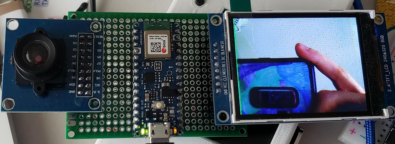
In areas that experience plenty of cold weather, icicles and ice dams can present a very real danger to the people and property nearby. In response, Eivind Holt has developed a computer vision-based system that relies on an Arduino Portenta H7, a Portenta Vision Shield, and a slew of AI tools/models to recognize this ice buildup. Best of all, the board’s low power consumption and LoRaWAN connectivity means it can be deployed almost anywhere outdoors.
Before a model can be created, it needs copious amounts of training, data which normally comes from manually-annotated, real images. But recent advancements have allowed for synthetic datasets to be used instead, such as with NVIDIA’s Omniverse Replicator. It was in here that Holt programmatically added a virtual house and randomized icicle models, as well as configured Omniverse to move the camera around a raytraced scene in order to snap virtual pictures and annotate them with the correct label.
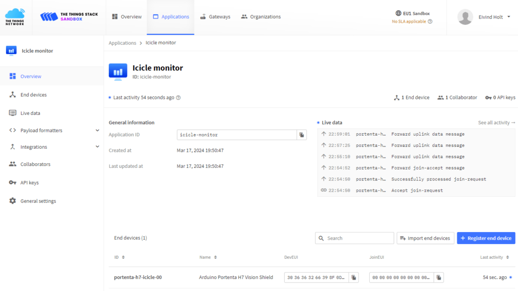
Once the realistic, synthetic data had been created, Holt exported everything to Edge Impulse and trained an object detection model for the Portenta H7, although it was also tested in NVIDIA’s Isaac Sim environment via the Edge Impulse extension prior to deployment. Alert generation was achieved by connecting the LoRaWAN radio to The Things Stack and sending a small, binary payload every ten seconds if any icicles were detected.
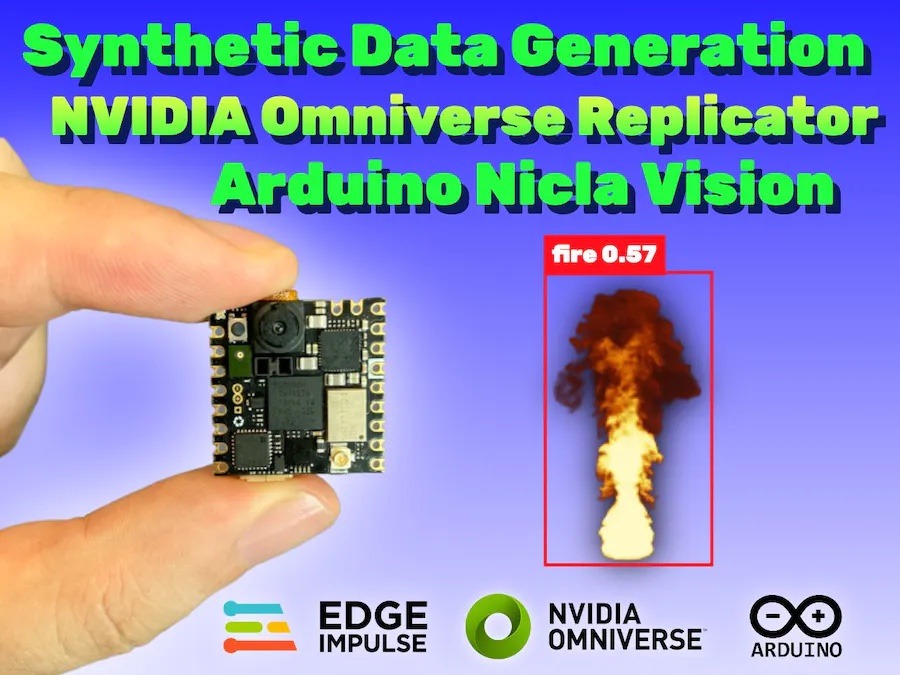
Due to an ever-warming planet thanks to climate change and greatly increasing wildfire chances because of prolonged droughts, being able to quickly detect when a fire has broken out is vital for responding while it’s still in a containable stage. But one major hurdle to collecting machine learning model datasets on these types of events is that they can be quite sporadic. In his proof of concept system, engineer Shakhizat Nurgaliyev shows how he leveraged NVIDIA Omniverse Replicator to create an entirely generated dataset and then deploy a model trained on that data to an Arduino Nicla Vision board.
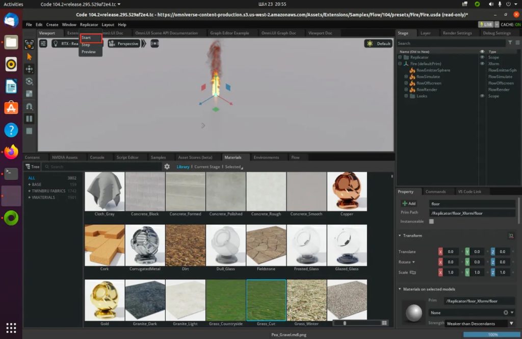
The project started out as a simple fire animation inside of Omniverse which was soon followed by a Python script that produces a pair of virtual cameras and randomizes the ground plane before capturing images. Once enough had been created, Nurgaliyev utilized the zero-shot object detection application Grounding DINO to automatically draw bounding boxes around the virtual flames. Lastly, each image was brought into an Edge Impulse project and used to develop a FOMO-based object detection model.
By taking this approach, the model achieved an F1 score of nearly 87% while also only needing a max of 239KB of RAM and a mere 56KB of flash storage. Once deployed as an OpenMV library, Nurgaliyev shows in his video below how the MicroPython sketch running on a Nicla Vision within the OpenMV IDE detects and bounds flames. More information about this system can be found here on Hackster.io.
Due to an ever-warming planet thanks to climate change and greatly increasing wildfire chances because of prolonged droughts, being able to quickly detect when a fire has broken out is vital for responding while it’s still in a containable stage. But one major hurdle to collecting machine learning model datasets on these types of events is that they can be quite sporadic. In his proof of concept system, engineer Shakhizat Nurgaliyev shows how he leveraged NVIDIA Omniverse Replicator to create an entirely generated dataset and then deploy a model trained on that data to an Arduino Nicla Vision board.
The project started out as a simple fire animation inside of Omniverse which was soon followed by a Python script that produces a pair of virtual cameras and randomizes the ground plane before capturing images. Once enough had been created, Nurgaliyev utilized the zero-shot object detection application Grounding DINO to automatically draw bounding boxes around the virtual flames. Lastly, each image was brought into an Edge Impulse project and used to develop a FOMO-based object detection model.
By taking this approach, the model achieved an F1 score of nearly 87% while also only needing a max of 239KB of RAM and a mere 56KB of flash storage. Once deployed as an OpenMV library, Nurgaliyev shows in his video below how the MicroPython sketch running on a Nicla Vision within the OpenMV IDE detects and bounds flames. More information about this system can be found here on Hackster.io.
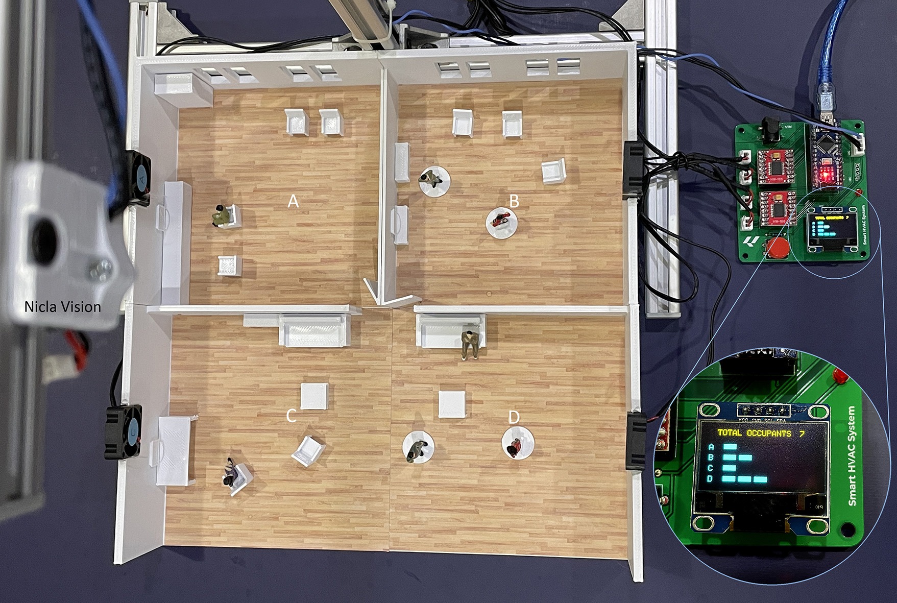
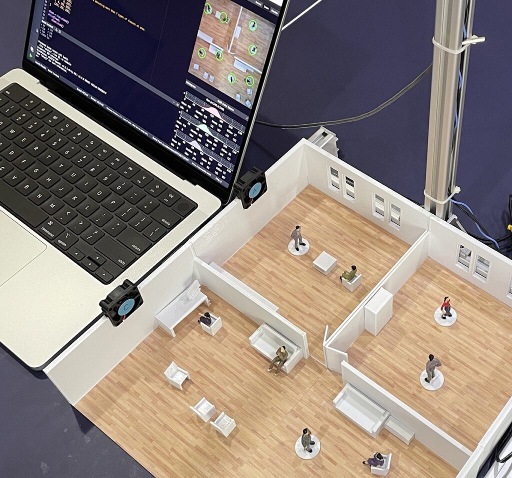
Shortly after setting the desired temperature of a room, a building’s HVAC system will engage and work to either raise or lower the ambient temperature to match. While this approach generally works well to control the local environment, the strategy also leads to tremendous wastes of energy since it is unable to easily adapt to changes in occupancy or activity. In contrast, Jallson Suryo’s smart HVAC project aims to tailor the amount of cooling to each zone individually by leveraging computer vision to track certain metrics.
Suryo developed his proof of concept as a 1:50 scale model of a plausible office space, complete with four separate rooms and a plethora of human figurines. Employing Edge Impulse and a smartphone, 79 images were captured and had bounding boxes drawn around each person for use in a FOMO-based object detection model. After training, Suryo deployed the OpenMV firmware onto an Arduino Nicla Vision board and was able to view detections in real-time.
The last step involved building an Arduino library containing the model and integrating it into a sketch that communicates with an Arduino Nano peripheral board over I2C by relaying the number of people per quadrant. Based on this data, the Nano dynamically adjusts one of four 5V DC fans to adjust the temperature while displaying relevant information on an OLED screen. To see how this POC works in more detail, you can visit Suryo’s write-up on the Edge Impulse docs page.
Maintaining accurate records for both the quantities and locations of inventory is vital when running any business operations efficiently and at scale. By leveraging new technologies such as AI and computer vision, items in warehouses, store shelves, and even a customer’s hand can be better managed and used to forecast changes demand. As demonstrated by the Zalmotek team, a tiny Arduino Nicla Vision board can be tasked with recognizing different types of containers and sending the resulting data to the cloud automatically.
The hardware itself was quite simple, as the Nicla Vision already contained the processor, camera, and connectivity required for the proof-of-concept. Once configured, Zalmotek used the OpenMV IDE to collect a large dataset featuring images of each type of item. Bounding boxes were then drawn using the Edge Impulse Studio, after which a FOMO-specific MobileNetV2 0.35 model was trained and could accurately determine the locations and quantities of objects in each test image.
Deploying the model was simple thanks to the OpenMV firmware export option, as it could be easily incorporated into the main Python script. In essence, the program continually gathers new images, passes them to the model, and gets the number of detected objects. Afterwards, these counts are published via the MQTT protocol to a cloud service for remote viewing.
It seems like most narrative games have some kind of drudgery built in. You know, some tedious and repetitious task that you absolutely must do if you want to succeed. In Stardew Valley, that thing is gift giving, which earns you friendship points just like in real life. More important than the giving itself is that each villager has preferences — things they love, like, and hate to receive as gifts. It’s a lot to remember, and most people don’t bother trying and just look it up in the wiki. Well, except for Abigail, who seems to like certain gemstones so much that she must be eating them. She’s hard to forget.
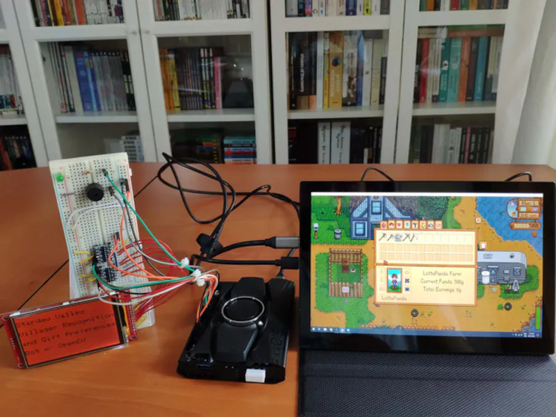
[kutluhan_aktar]’s villager gift preferences bot is a fun and fantastic use of OpenCV. This bot uses a LattePanda Alpha 864s, which is a single-board computer with an Arduino Leonardo built in. It works using template matching, which is basically a game of Where’s Waldo? for computers.
Given a screenshot of each villager in various positions, the LattePanda recognizes them among a given game scene, then does a lookup of their birthday and preferences which the Leonardo prints on a 3.5″ LCD screen. At the same time, it alerts the player with a buzz and big green LED. Be sure to check it out in action after the break.
The fantastical world of wizards and magic is one that can be explored by reading a book, and what better way to represent this than building your very own interactive diorama within a reading corner? Well, that is exactly what Andy of element14 Presents created when he combined a small display, computer vision, and LED lights into a fun bookshelf adornment, which would accompany readers on their journeys.
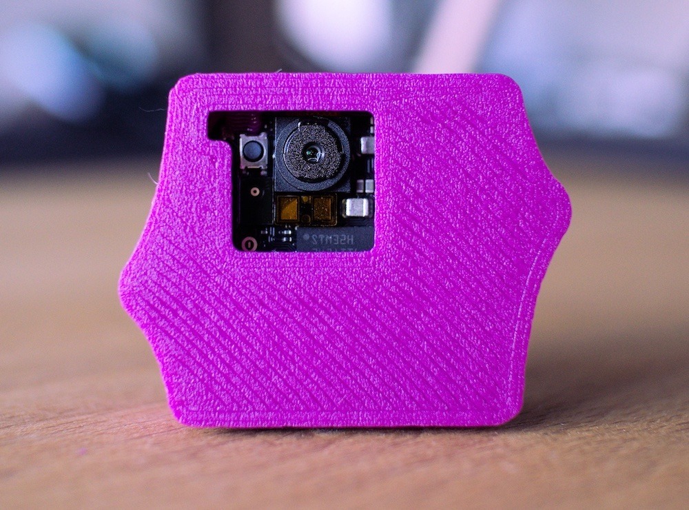
To begin, Andy had to figure out how to get a computer vision system into a space that is no larger than a shoebox, and for this task, he settled on using the Portenta H7 board plus its Vision Shield to gather images and classify them. His attempts to integrate a string of NeoPixels and an ePaper display module with MicroPython were unsuccessful, so this required a switch to only using C with TensorFlow Lite and some custom functions to take the framebuffers from the camera and determine if a face is present.
The diorama models themselves were fashioned from cardboard model railway kits that included houses and a few streetlights. Finally, the LEDs were added both behind the houses and inside of each lamppost that allows them to flicker and light up when a person is watching the display. The ePaper module switches between various stills such as a wanted poster and the element14 logo.
To see more about how this diorama was constructed, check out Andy’s video below!
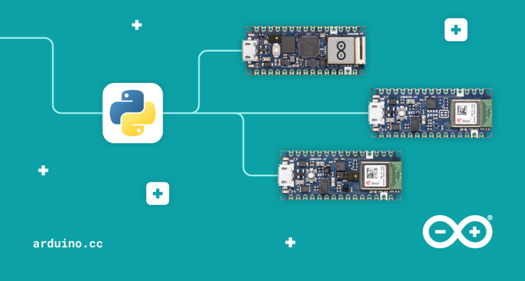
Python support for three of the hottest Arduino boards out there is now yours. Through our partnership with OpenMV, the Nano RP2040 Connect, Nano 33 BLE and Nano 33 BLE Sense can now be programmed with the popular MicroPython language. Which means you get OpenMV’s powerful computer vision and machine learning capabilities thrown in.
OpenMV IDE and MicroPython Editor
While you can’t use Python directly with the Arduino IDE, you can use the OpenMV editor, and its version of MicroPython. From the editor, you can install MicroPython and load your scripts directly to the supported Arduino boards.
MicroPython is a great implementation of the full Python programming language, designed to run on microcontrollers. There’s extensive documentation all across the web, which is another huge advantage of learning and using Python for your Arduino projects.
There are so many reasons to get excited about MicroPython for these new Arduino boards. To name a few…
OpenMV’s machine learning and computer vision tools.
Great for computer science education.
Easy for web developers and coders to switch from other platforms to Arduino.
Huge number of MicroPython libraries, tutorials, guides and support online.
Simple to upgrade hardware as project demands increase (eg, upgrade from a Nano RP2040 Connect to a Portenta H7).
There are also lots of Arduino + Python projects that have been posted over the years. Now you can add the Nano devices to those projects and expand on them with their new MicroPython capabilities.
Get Started with Python on Arduino
To help you get cracking, we’ve put together a few guides for each of the supported Arduino boards. The Portanta H7 already supports MicroPython, but we’ve included it below for the sake of completion.
If it’s the first time you’ve used Python on your Arduino board, you’ll need to follow a few steps to get everything working together. Depending on which board you’re using, you might need to update the bootloader to make it compatible with OpenMV. Then you can connect to the board to upload the latest firmware and make it compatible with the editor.
There are guides to take you through the process for each board, and it’s not a complex task. Once completed, your boards will be ready to program them using MicroPython.
These simple tutorials will get you moving quickly.
Furthermore, you can find a few examples of MicroPython scripts you can upload and run on the various boards, too. It’s a great way to test the Python waters with your Arduino boards, and pick up a couple of hints and tips on using the language.
If you’ve got any resources, hints or tips of your own when it comes to learning or using Python, please do share them with the community! We want to hear all about your experiences, and any projects you build using Arduino and Python together.
We’ll keep you updated as we add more documentation and tutorials for MicroPython over on Arduino Docs, so keep an eye out for those.
In this deep dive article, performance optimization specialist Larry Bank (a.k.a The Performance Whisperer) takes a look at the work he did for the Arduino team on the latest version of the Arduino_OV767x library.
Arduino recently announced an update to the Arduino_OV767x camera library that makes it possible to run machine vision using TensorFlow Lite Micro on your Arduino Nano 33 BLE board.
If you just want to try this and run machine learning on Arduino, you can skip to the project tutorial.
The rest of this article is going to look at some of the lower level optimization work that made this all possible. There are higher performance industrial-targeted options like the Arduino Portenta available for machine vision, but the Arduino Nano 33 BLE has sufficient performance with TensorFlow Lite Micro support ready in the Arduino IDE. Combined with an OV767x module makes a low-cost machine vision solution for lower frame-rate applications like the person detection example in TensorFlow Lite Micro.
Need for speed
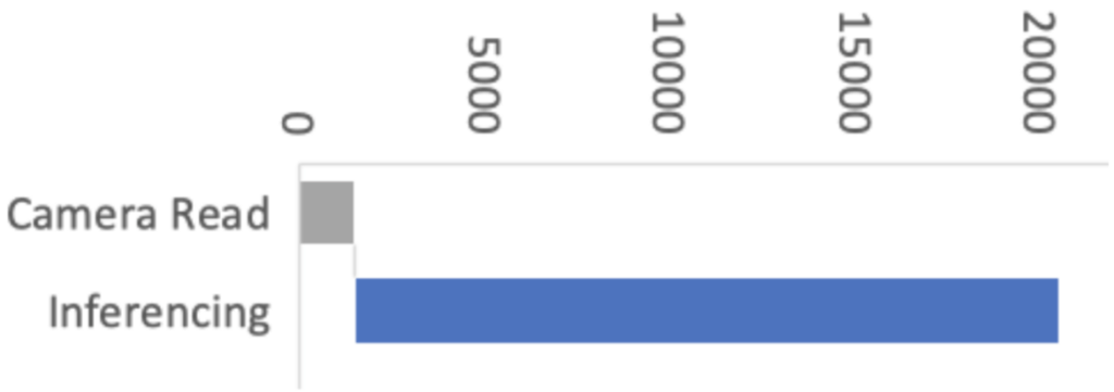
Recent optimizations done by Google and Arm to the CMSIS-NN library also improved the TensorFlow Lite Micro inference speed by over 16x, and as a consequence bringing down inference time from 19 seconds to just 1.2 seconds on the Arduino Nano 33 BLE boards. By selecting the person_detection example in the Arduino_TensorFlowLite library, you are automatically including CMSIS-NN underneath and benefitting from these optimizations. The only difference you should see is that it runs a lot faster!
The CMSIS-NN library provides optimized neural network kernel implementations for all Arm’s Cortex-M processors, ranging from Cortex-M0 to Cortex-M55. The library utilizes the processor’s capabilities, such as DSP and M-Profile Vector (MVE) extensions, to enable the best possible performance.
The Arduino Nano 33 BLE board is powered by Arm Cortex-M4, which supports DSP extensions. That will enable the optimized kernels to perform multiple operations in one cycle using SIMD (Single Instruction Multiple Data) instructions. Another optimization technique used by the CMSIS-NN library is loop unrolling. These techniques combined will give us the following example where the SIMD instruction, SMLAD (Signed Multiply with Addition), is used together with loop unrolling to perform a matrix multiplication y=a*b, where
a=[1,2]
and
  b=[3,5
     4,6]
a, b are 8-bit values and y is a 32-bit value. With regular C, the code would look something like this:
However, using loop unrolling and SIMD instructions, the loop will end up looking like this:
a_operand = a[0] | a[1] << 16 // put a[0], a[1] into one variable
  for(i=0; i<2; ++i)
    b_operand = b[0][i] | b[1][i] << 16 // vice versa for b
    y[i] = __SMLAD(a_operand, b_operand, y[i])
This code will save cycles due to
fewer for-loop checks
__SMLAD performs two multiply and accumulate in one cycle
This is a simplified example of how two of the CMSIS-NN optimization techniques are used.
Figure 1: Performance with initial versions of libraries
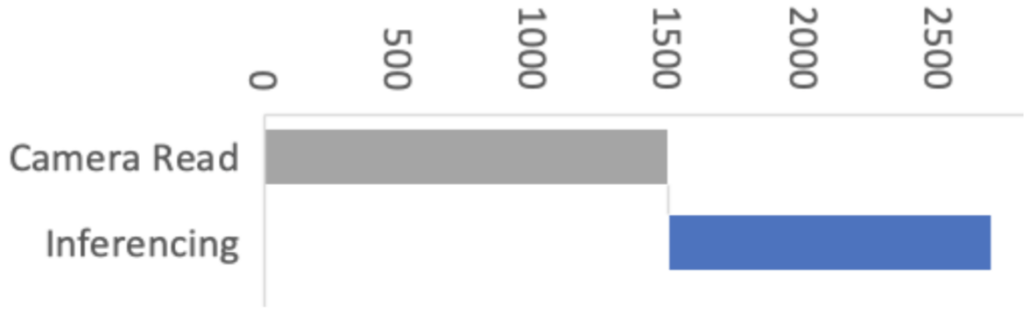
Figure 2: Performance with CMSIS-NN optimizations
This improvement means the image acquisition and preprocessing stages now have a proportionally bigger impact on machine vision performance. So in Arduino our objective was to improve the overall performance of machine vision inferencing on Arduino Nano BLE sense by optimizing the Arduino_OV767X library while maintaining the same library API, usability and stability.
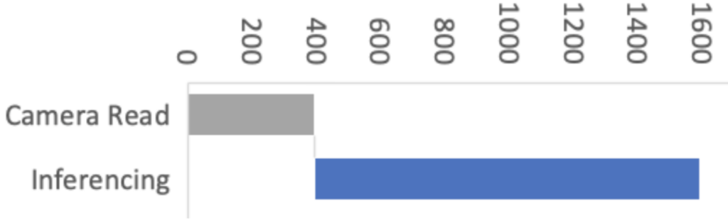
Figure 3: Performance with CMSIS-NN and camera library optimizations
For this, we enlisted the help of Larry Bank who specializes in embedded software optimization. Larry’s work got the camera image read down from 1500ms to just 393ms for a QCIF (176×144 pixel) image. This was a great improvement!
Let’s have a look at how Larry approached the camera library optimization and how some of these techniques can apply to your Arduino code in general.
Performance optimizing Arduino code
It’s rarely practical or necessary to optimize every line of code you write. In fact there are very good reasons to prioritize readable, maintainable code. Being readable and optimized don’t necessarily have to be mutually exclusive. However, embedded systems have constrained resources, and when applications demand more performance, some trade-offs might have to be made. Sometimes it is necessary to restructure algorithms, pay attention to compiler behavior, or even analyze timing of machine code instructions in order to squeeze the most out of a microcontroller. In some cases this can make the code less readable — but the beauty of an Arduino library is that this can be abstracted (hidden) from user sketch code beneath the cleaner library function APIs.
What does “Camera.readFrame” do?
We’ve connected a camera to the Arduino. The Arduino_OV767X library sets up the camera and lets us transfer the raw image data from the camera into the Arduino Nano BLE memory. The smallest resolution setting, QCIF, is 176 x 144 pixels. Each pixel is encoded in 2 bytes. We therefore need to transfer at least 50688 bytes (176 x 144 x 2 ) every time we capture an image with Camera.readFrame. Because the function is performing a byte read operation over 50 thousand times per frame, the way it’s implemented has a big impact on performance. So let’s have a look at how we can most efficiently connect the camera to the Arduino and read a byte of data from it.
Philosophy
I tend to see the world of code through the “lens” of optimization. I’m not advocating for everyone to share my obsession with optimization. However, when it does become necessary, it’s helpful to understand details of the target hardware and CPU. What I often encounter with my clients is that their code implements their algorithm neatly and is very readable, but it’s not necessarily ‘performance friendly’ to the target machine. I assume this is because most people see code from a top-down approach: they think in terms of the abstract math and how to process the data. My history in working with very humble machines and later turning that into a career has flipped that narrative on its head. I see software from the bottom up: I think about how the memory, I/O and CPU registers interact to move and process the data used by the algorithm. It’s often possible to make dramatic improvements to the code execution speed without losing any of its readability. When your readable/maintainable solution still isn’t fast enough, the next phase is what I call ‘uglification.’ This involves writing code that takes advantage of specific features of the CPU and is nearly always more difficult to follow (at least at first glance!).
Optimization methodology
Optimization is an iterative process. I usually work in this order:
Test assumptions in the algorithm (sometimes requires tracing the data)
Make innocuous changes in the logic to better suit the CPU (e.g. change modulus to logical AND)
Flatten the hierarchy or simplify overly nested classes/structures
Test any slow/fast paths (aka statistics of the data — e.g. is 99% of the incoming data 0?)
Go back to the author(s) and challenge their decisions on data precision / storage
Make the code more suitable for the target architecture (e.g. 32 vs 64-bit CPU registers)
If necessary (and permitted by the client) use intrinsics or other CPU-specific features
Go back and test every assumption again
If you would like to investigate this topic further, I’ve written a more detailed presentation on Writing Performant C++ code.
Depending on the size of the project, sometimes it’s hard to know where to start if there are too many moving parts. If a profiler is available, it can help narrow the search for the “hot spots” or functions which are taking the majority of the time to do their work. If no profiler is available, then I’ll usually use a time function like micros() to read the current tick counter to measure execution speed in different parts of the code. Here is an example of measuring absolute execution time on Arduino:
long lTime;
  lTime = micros();
  <do the work>
  iTime = micros() - lTime;
  Serial.printf(“Time to execute xxx = %d microseconds\n”, (int)lTime);
I’ve also used a profiler for my optimization work with OpenMV. I modified the embedded C code to run as a MacOS command line app to make use of the excellent XCode Instruments profiler. When doing that, it’s important to understand how differently code executes on a PC versus embedded — this is mostly due to the speed of the CPU compared to the speed of memory.
Pins, GPIO and PORTs
One of the most powerful features of the Arduino platform is that it presents a consistent API to the programmer for accessing hardware and software features that, in reality, can vary greatly across different target architectures. For example, the features found in common on most embedded devices like GPIO pins, I2C, SPI, FLASH, EEPROM, RAM, etc. have many diverse implementations and require very different code to initialize and access them.
Let’s look at the first in our list, GPIO (General Purpose Input/Output pins). On the original Arduino Uno (AVR MCU), the GPIO lines are arranged in groups of 8 bits per “PORT” (it’s an 8-bit CPU after all) and each port has a data direction register (determines if it’s configured for input or output), a read register and a write register. The newer Arduino boards are all built around various Arm Cortex-M microcontrollers. These MCUs have GPIO pins arranged into groups of 32-bits per “PORT” (hmm – it’s a 32-bit CPU, I wonder if that’s the reason). They have a similar set of control mechanisms, but add a twist — they include registers to SET or CLR specific bits without disturbing the other bits of the port (e.g. port->CLR = 1; will clear GPIO bit 0 of that port). From the programmer’s view, Arduino presents a consistent set of functions to access these pins on these diverse platforms (clickable links below to the function definitions on Arduino.cc):
For me, this is the most powerful idea of Arduino. I can build and deploy my code to an AVR, a Cortex-M, ESP8266 or an ESP32 and not have to change a single line of code nor maintain multiple build scripts. In fact, in my daily work (both hobby and professional), I’m constantly testing my code on those 4 platforms. For example, my LCD/OLED display library (OneBitDisplay) can control various monochrome LCD and OLED displays and the same code runs on all Arduino boards and can even be built on Linux.
One downside to having these ‘wrapper’ functions hide the details of the underlying implementation is that performance can suffer. For most projects it’s not an issue, but when you need to get every ounce of speed out of your code, it can make a huge difference.
Camera data capture
One of the biggest challenges of this project was that the original OV7670 library was only able to run at less than 1 frame per second (FPS) when talking to the Nano 33. The reason for the low data rate is that the Nano 33 doesn’t expose any hardware which can directly capture the parallel image data, so it must be done ‘manually’ by testing the sync signals and reading the data bits through GPIO pins (e.g. digitalRead) using software loops. The Arduino pin functions (digitalRead, digitalWrite) actually contain a lot of code which checks that the pin number is valid, uses a lookup table to convert the pin number to the I/O port address and bit value and may even disable interrupts before reading or changing the pin state. If we were to use the digitalRead function for an application like this, it would limit the data capture rate to be too slow to operate the camera. You’ll see this further down when we examine the actual code used to capture the data.
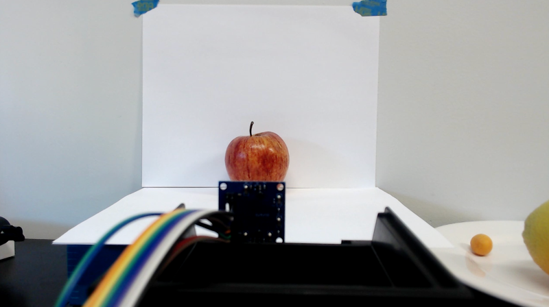
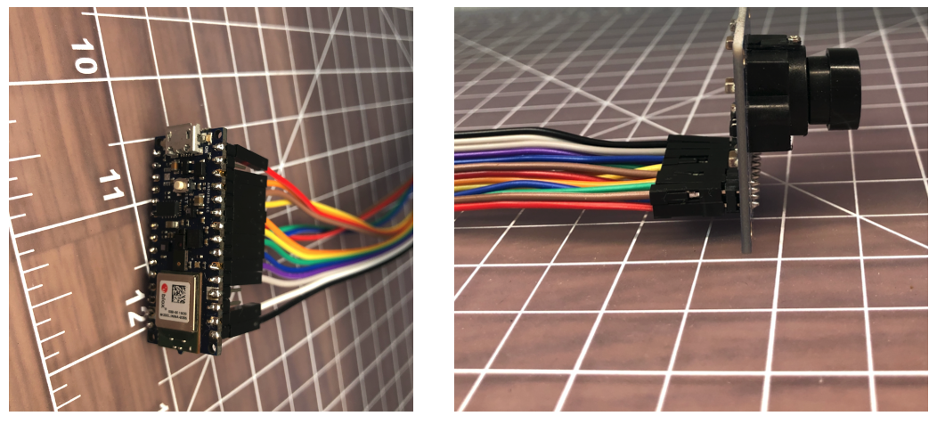
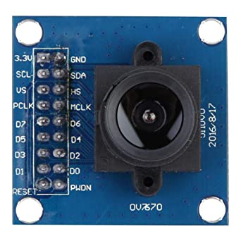
First, a quick review of the OV7670 camera module: According to its datasheet, it’s capable of capturing a VGA (640×480) color image at up to 30 FPS. The kit used for this project has the camera mounted to a small PCB and presents an 8-bit parallel data bus and various sync signals.
It requires an external “master clock” (MCLK in the photo) to drive its internal state machine which is used to generate all of the other timing signals. The Nano 33 can provide this external clock source by using its I2S clock. The OV767X library sets this master clock to 16Mhz (the camera can handle up to 48Mhz) and then there is a set of configuration registers to divide this value to arrive at the desired frame rate. Only a few possible frame rates are available (1, 5, 10, 15, 20, and 30 FPS).
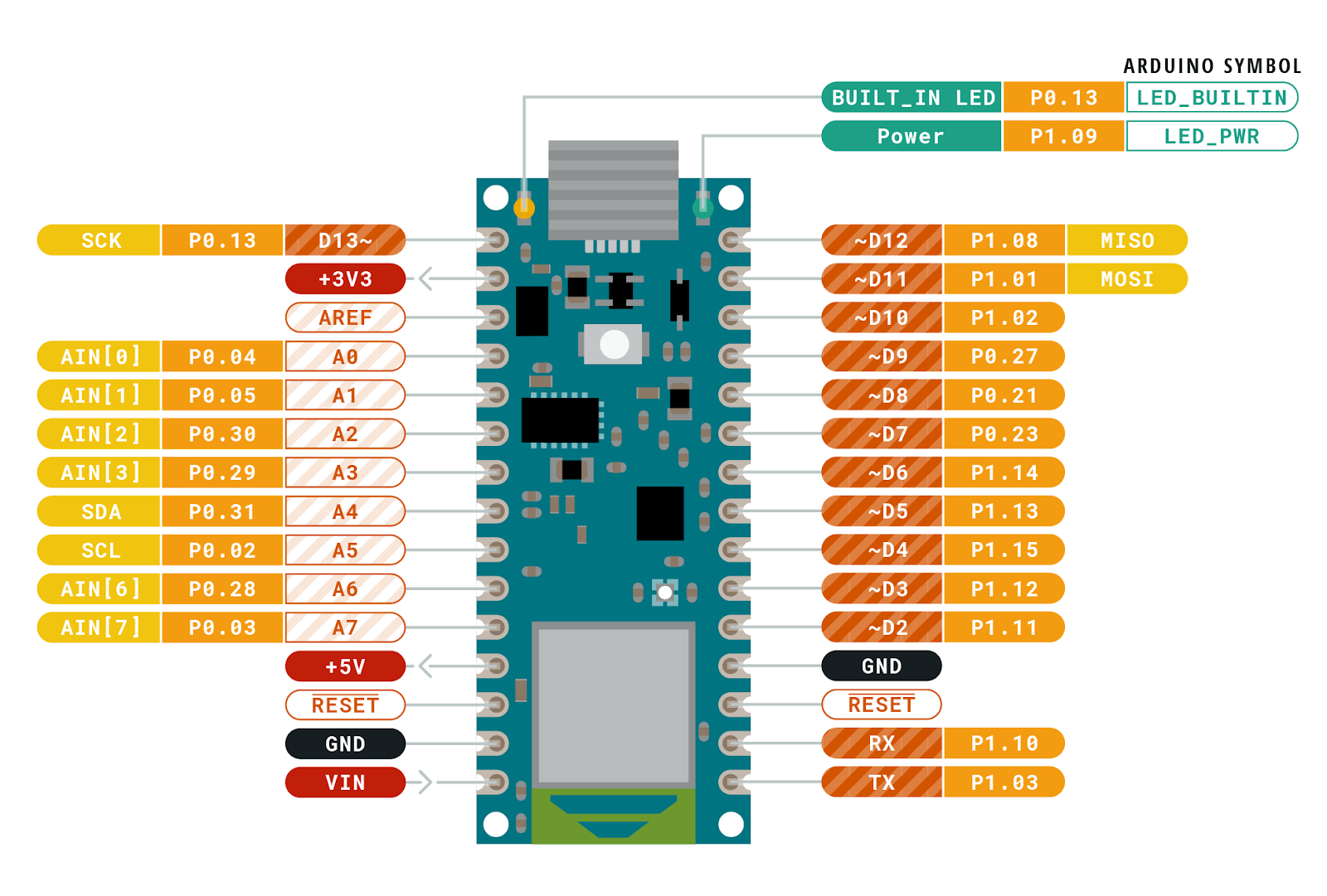
Above is one of the timing diagrams from the OV7670 datasheet. This particular drawing shows the timing of the data for each byte received along each image row. The HREF signal is used to signal the start and end of a row and then each byte is clocked in with the PCLK signal. The original library code read each bit (D0-D7) in a loop and combined them together to form each data byte. The image data comes quickly, so we have very little time to read each byte. Assembling them one bit at a time is not very efficient. You might be thinking that it’s not that hard of a problem to solve on the Nano 33. After all, it has 22 GPIO pins and the Cortex-M inside it has 32-bit wide GPIO ports, so just hook up the data bits sequentially and you’ll be able to read the 8 data bits in one shot, then Mission Accomplished. If only things were that easy. The Nano 33 does have plenty of GPIO pins, but there isn’t a continuous sequence of 8 bits available using any of the pins! I’m guessing that the original code did it one bit at a time because it didn’t look like there was a better alternative. In the pinout diagram below, please notice the P0.xx and P1.xx numbers. These are the Cortex-M GPIO port 0 and 1-bit numbers (other Cortex-M processors would label them PA and PB).
I wasn’t going to let this little bump in the road stop me from making use of bit parallelism. If you look carefully at the bit positions, the best continuous run we can get is 6 bits in a row with P1.10 through P1.15. It’s not possible to read the 8 data bits in one shot…or is it? If we connect D0/D1 of the camera to P1.02/P1.03 and D2-D7 to P1.10-P1.15, we can do a single 32-bit read from port P1 and get all 8 bits in one shot. The bits are in order, but will have a gap between D1 and D2 (P1.04 to P1.09). Luckily the Arm CPU has what’s called a barrel shifter. It also has a smart instruction set which allows data to be shifted ‘for free’ at the same time the instruction is doing something else. Let’s take a look at how and why I changed the code:
Original:
uint8_t in = 0;
  for (int k = 0; k < 8; k++) {
     bitWrite(in, k, (*_dataPorts[k] & _dataMasks[k]) != 0);
  }
Optimized:
  uint32_t in = port->IN; // read all bits in parallel
  in >>= 2; // place bits 0 and 1 at the "bottom" of the
register
  in &= 0x3f03; // isolate the 8 bits we care about
  in |= (in >> 6); // combine the upper 6 and lower 2 bits
Code analysis
If you’re not interested in the nitty gritty details of the code changes I made, you can skip this section and go right to the results below.First, let’s look at what the original code did. When I first looked at it, I didn’t recognize bitWrite; apparently it’s not a well known Arduino bit manipulation macro; it’s defined as:
This macro was written with the intention of being used on GPIO ports (the variable value) where the logical state of bitvalue would be turned into a single write of a 0 or 1 to the appropriate bit. It makes less sense to be used on a regular variable because it inserts a branch to switch between the two possible outcomes. For the task at hand, it’s not necessary to use bitClear() on the in variable since it’s already initialized to 0 before the start of each byte loop. A better choice would be:
if (*_dataPorts[k] & _dataMasks[k]) in |= (1 << k);
The arrays _dataPorts[] and _dataMasks[] contain the memory mapped GPIO port addresses and bit masks to directly access the GPIO pins (bypassing digitalRead). So here’s a play-by-play of what the original code was doing:
Set in to 0
Set k to 0
Read the address of the GPIO port from _dataPorts[] at index k
Read the bit mask of the GPIO port from _dataMasks[] at index k
Read 32-bit data from the GPIO port address
Logical AND the data with the mask
Shift 1 left by k bits to prepare for bitClear and bitSet
Compare the result of the AND to zero
Branch to bitSet() code if true or use bitClear() if false
bitClear or bitSet depending on the result
Increment loop variable k
Compare k to the constant value 8
Branch if less back to step 3
Repeat steps 3 through 13, 8 times
Store the byte in the data array (not shown above)
The new code does the following:
Read the 32-bit data from the GPIO port address
Shift it right by 2 bits
Logical AND (mask) the 8 bits we’re interested in
Shift and OR the results to form 8 continuous bits
Store the byte in the data array (not shown above)
Each of the steps listed above basically translates into a single Arm instruction. If we assume that each instruction takes roughly the same amount of time to execute (mostly true on Cortex-M), then old vs. new is 91 versus 5 instructions to capture each byte of camera data, an 18x improvement! If we’re capturing a QVGA frame (320x240x2 = 153600 bytes), that becomes manymillionsof extra instructions.
Results
The optimized byte capture code translates into 5 Arm instructions and allows the capture loop to now handle a setting of 5 FPS instead of 1 FPS. The FPS numbers don’t seem to be exact, but the original capture time (QVGA @ 1 FPS) was 1.5 seconds while the new capture time when set to 5 FPS is 0.393 seconds. I tested 10 FPS, but readFrame() doesn’t read the data correctly at that speed. I don’t have an oscilloscope handy to probe the signals to see why it’s failing. The code may be fast enough now (I think it is), but the sync signals may become too unstable at that speed. I’ll leave this as an exercise to the readers who have the equipment to see what happens to the signals at 10 FPS.
For the work I did on the OV767X library, I created a test fixture to make sure that the camera data was being received correctly. For ML/data processing applications, it’s not necessary to do this. The built-in camera test pattern can be used to confirm the integrity of the data by using a CRC32.
My tinned protoboard test fixture with 320×240 LCD
Note: The frames come one immediately after another. If you capture a frame and then do some processing and then try to capture another frame, you may hit the middle of the next frame when you call readFrame(). The code will then wait until the next VSync signal, so that frame’s capture time could be as much as 2x as long as a single frame time.
More tips
I enjoy testing the limits of embedded hardware, especially when it involves bits, bytes and pixels. I’ve written a few blog posts that explore the topics of speed and power usage if you’re interested in learning more about it.
Conclusion
The embedded microcontrollers available today are capable of handling jobs that were unimaginable just a few years ago.
Optimized ML solutions from Google and Edge Impulse are capable of running on low-cost, battery-powered boards (vision, vibration, audio, whatever sensor you want to monitor).
Python and Arduino programming environments can test your project idea with little effort.
Software can be written an infinite number of ways to accomplish the same task, but one constant remains: TANSTATFC (there ain’t no such thing as the fastest code).
Never assume the performance you’re seeing is what you’re stuck with. Think of existing libraries and generic APIs available through open source libraries and environments as a starting point.
Knowing a bit of info about the target platform can be helpful, but it’s not necessary to read the MCU datasheet. In the code above, the larger concept of Arm Cortex-M 32-bit GPIO ports was sufficient to accomplish the task without knowing the specifics of the nRF52’s I/O hardware.
Don’t be afraid to dig a little deeper and test every assumption.
If you encounter difficulties, the community is large and there are a ton of resources out there. Asking for help is a sign of strength, not weakness.
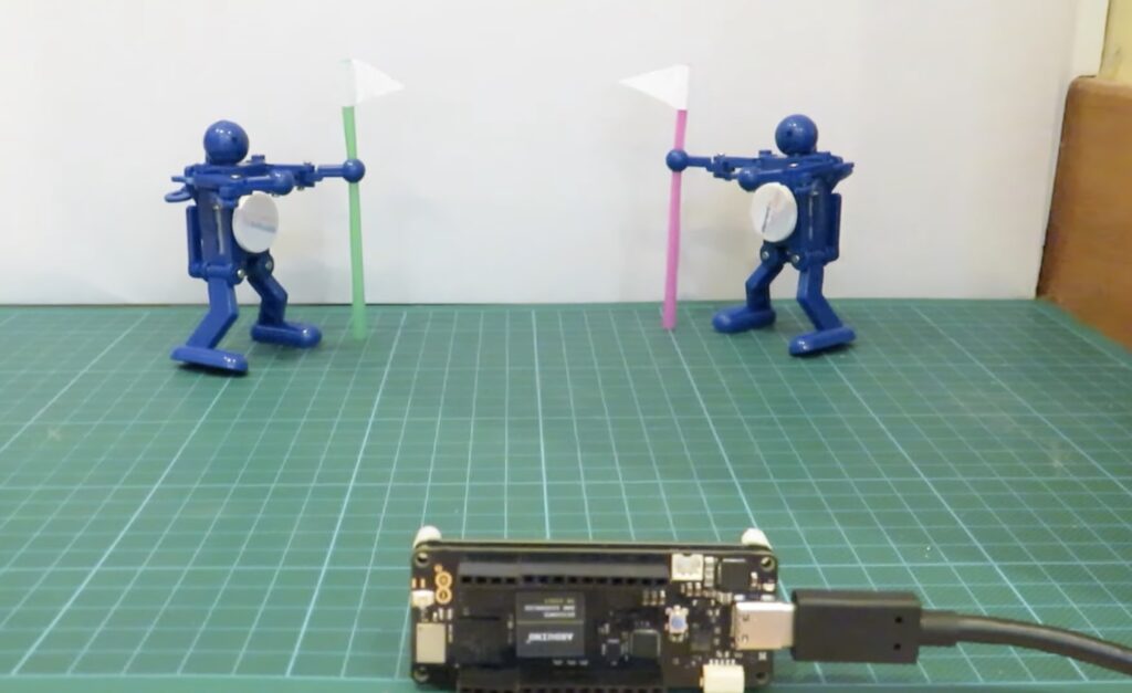
Ever since he was a young boy, [Tyler] has played the silver ball. And like us, he’s had a lifelong fascination with the intricate electromechanical beasts that surround them. In his recently-completed senior year of college, [Tyler] assembled a mechatronics dream team of [Kevin, Cody, and Omar] to help turn those visions into self-playing pinball reality.
You can indeed play the machine manually, and the Arduino Mega will keep track of your score just like a regular cabinet. If you need to scratch an itch, ignore a phone call, or just plain want to watch a pinball machine play itself, it can switch back and forth on the fly. The USB camera mounted over the playfield tracks the ball as it speeds around. Whenever it enters the flipper vectors, the appropriate flipper will engage automatically to bat the ball away.
Our favorite part of this build (aside from the fact that it can play itself) is the pachinko multi-ball feature that manages to squeeze in a second game and a second level. This project is wide open, and even if you’re not interested in replicating it, [Tyler] sprinkled a ton of good info and links to more throughout the build logs. Take a tour after the break while we have it set on free play.
Planet Arduino is, or at the moment is wishing to become, an aggregation of public weblogs from around the world written by people who develop, play, think on Arduino platform and his son. The opinions expressed in those weblogs and hence this aggregation are those of the original authors. Entries on this page are owned by their authors. We do not edit, endorse or vouch for the contents of individual posts. For more information about Arduino please visit www.arduino.cc
You are currently browsing the archives for the computer vision category.


 . If only things were that easy. The Nano 33 does have plenty of GPIO pins, but there isn’t a continuous sequence of 8 bits available using any of the pins! I’m guessing that the original code did it one bit at a time because it didn’t look like there was a better alternative. In the pinout diagram below, please notice the P0.xx and P1.xx numbers. These are the Cortex-M GPIO port 0 and 1-bit numbers (other Cortex-M processors would label them PA and PB).