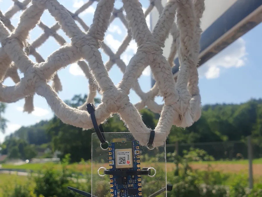
When playing a short game of basketball, few people enjoy having to consciously track their number of successful throws. Yet when it comes to automation, nearly all systems rely on infrared or visual proximity detection as a way to determine when a shot has gone through the basket versus missed. This is what inspired one team from the University of Ljubljan to create a small edge ML-powered device that can be suspended from the net with a pair of zip ties for real-time scorekeeping.
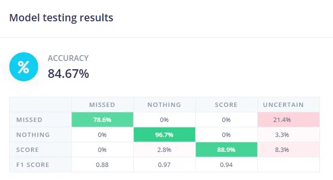
After collecting a total of 137 accelerometer samples via an Arduino Nano 33 BLE Sense and labeling them as either a miss, a score, or nothing within the Edge Impulse Studio, the team trained a classification model and reached an accuracy of 84.6% on real-world test data. Getting the classification results from the device to somewhere readable is handled by the Nano’s onboard BLE server. It provides two services, with the first for reporting the current battery level and the second for sending score data.
Once the firmware had been deployed, the last step involved building a mobile application to view the relevant information. The app allows users to connect to the basketball scoring device, check if any new data has been received, and then parse/display the new values onscreen.
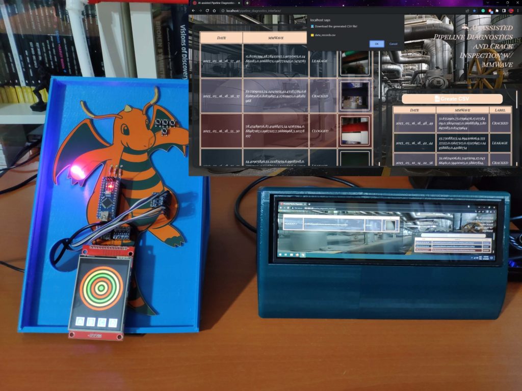
Pipelines are integral to our modern way of life, as they enable the fast transportation of water and energy between central providers and the eventual consumers of that resource. However, the presence of cracks from mechanical or corrosive stress can lead to leaks, and thus waste of product or even potentially dangerous situations. Although methods using thermal cameras or microphones exist, they’re hard to use interchangeably across different pipeline types, which is why Kutluhan Aktar instead went with a combination of mmWave radar and an ML model running on an Arduino Nicla Vision board to detect these issues.
The project was originally conceived as an arrangement of parts on a breadboard, including a Seeed Studio MR60BHA1 60GHz radar module, an ILI9341 TFT screen, an Arduino Nano for interfacing with the sensor and display, and a Nicla Vision board. From here, Kutluhan designed his own Dragonite-themed PCB, assembled the components, and began collecting training and testing data for a machine learning model by building a small PVC model, introducing various defects, and recording the differences in data from the mmWave sensor.
After configuring a time-series impulse, a classification model was trained with the help of Edge Impulse and then deployed to the Nicla Vision where it achieved an accuracy of 90% on real-world data. With the aid of the display, operators can tell the result of the classification immediately, as well as send the data to a custom web application.
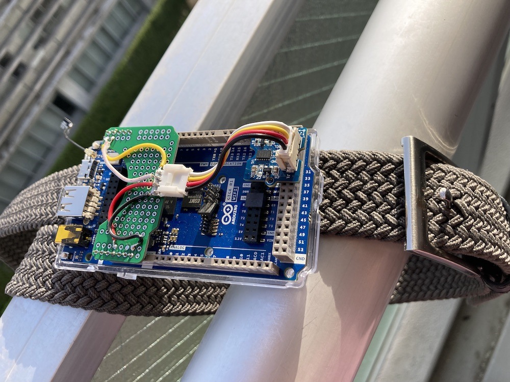
For those aged 65 and over, falls can be one of the most serious health concerns they face either due to lower mobility or decreasing overall coordination. Recognizing this issue, Naveen Kumar set out to produce a wearable fall-detecting device that aims to increase the speed at which this occurs by utilizing a Transformer-based model rather than a more traditional recurrent neural network (RNN) model.
Because this project needed to be both fast and consume only small amounts of current, Kumar went with the new Arduino GIGA R1 WiFi due to its STM32H74XI dual-core Arm CPU, onboard WiFi/Bluetooth®, and ability to interface with a wide variety of sensors. After connecting an ADXL345 three-axis accelerometer, he realized that collecting many hours of samples by hand would be far too time consuming, so instead, he downloaded the SisFall dataset, ran a Python script to parse the sample data into an Edge Impulse-compatible format, and then uploaded the resulting JSON files into a new project. Once completed, he used the API to split each sample into four-second segments and then used the Keras block edit feature to build a reduced-sized Transformer model.
The result after training was a 202KB large model that could accurately determine if a fall occurred 96% of the time. Deployment was then as simple as using the Arduino library feature within a sketch to run an inference and display the result via an LED, though future iterations could leverage the GIGA R1 WiFi’s connectivity to send out alert notifications if an accident is detected. More information can be found here in Kumar’s write-up.
Wevolver’s previous article about the Arduino Pro ecosystem outlined how embedded sensors play a key role in transforming machines and automation devices to Cyber Physical Production Systems (CPPS). Using CPPS systems, manufacturers and automation solution providers capture data from the shop floor and use it for optimizations in areas like production schedules, process control, and quality management. These optimizations leverage advanced data Internet of Things (IoT) analytics over manufacturing datasets, which is the reason why data are the new oil.
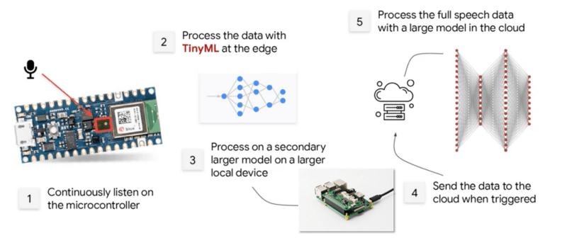
Deployment Options for IoT Analytics: From Cloud Analytics to TinyML
IoT analytics entail statistical data processing and employ Machine Learning (ML) functions, including Deep Learning (DL) techniques i.e., ML based on deep neural networks. Many manufacturing enterprises deploy IoT analytics in the cloud. Cloud IoT analytics use the vast amounts of cloud data to train accurate DL models. Accuracy is important for many industrial use cases like Remaining Useful Life calculation in predictive maintenance. Nevertheless, it is also possible to execute analytics at the edge of the network. Edge analytics are deployed within embedded devices or edge computing clusters at the factory’s Local Area Network (LAN). They are appropriate for real-time use cases that demand low latency such as real-time detection of defects. Edge analytics are more power-efficient than cloud analytics. Moreover, they offer increased data protection as data stays within the LAN.
During the last couple of years, industrial organizations use TinyML to execute ML models within CPU and memory-constrained devices. TinyML is faster, real-time, more power-efficient, and more privacy-friendly than any other form of edge analytics. Therefore, it provides benefits for many Industry 4.0 use cases.
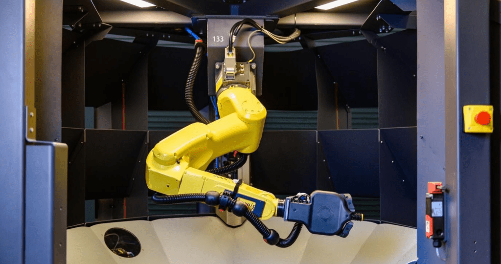
TinyML is the faster, real-time, most power-efficient, and most privacy friendly form of edge analytics. Image credit: Carbon Robotics.
Building TinyML Applications
The process of developing and deploying TinyML applications entails:
Getting or Producing a Dataset, which is used for training the TinyML model. In this direction, data from sensors or production logs can be used.
Train an ML or DL Model, using standard tools and libraries like Jupyter Notebooks and Python packages like TensorFlow and NumPy. The work entails Exploratory Data Analysis steps towards understanding the data, identifying proper ML models, and preparing the data for training them.
Evaluate the Model’s Performance, using the trained model predictions and calculating various error metrics Depending on the achieved performance, the TinyML engineer may have to improve the model and avoid overfitting on the data. Different models must be tested to find the best one.
Make the Model Appropriate to Run on an Embedded Device, using tools like TensorFlow Lite which provides a “converter” library that turns a model into a space-efficient format. TensorFlow Lite provides also an “interpreter” library that runs the converted model using the most efficient operations for a given device. In this step, a C/C++ sketch is produced to enable on device deployment.
On-device Inference and Binary Development, which involves the C/C++ and embedded systems development part and produces a binary application for on-device inference.
Deploying the Binary to a Microcontroller, which makes the microcontroller able to analyse data and derive real-time insights.
Building a Google Assistant using tinyML. Image credit: Arduino.
Leveraging AutoML for Faster Development with Arduino Pro
Nowadays, Automatic Machine Learning (AutoML) tools are used to develop TinyML on various boards, including Arduino boards. Emerging platforms such as Edge Impulse, Qeexo and SensiML, among others, provide AutoML tools and developers’ resources for embedded ML development. Arduino is collaborating with such platforms as part of their strategy to make complex technologies open and simple to use by anyone.
Within these platforms, users collect real-world sensor data, train ML models on the cloud, and ultimately deploy the model back to an Arduino device. It is also possible to integrate ML models with Arduino sketches based on simple function calls. AutoML pipelines ease the tasks of (re)developing and (re)deploying models to meet complex requirements.
The collaboration between Arduino and ML platforms enables thousands of developers to build applications that embed intelligence in smart devices such as applications that recognize spoken keywords, gestures, and animals. Implementing applications that control IoT devices via natural language or gestures is relatively straightforward for developers who are familiar with Arduino boards.
Arduino has recently introduced its new Arduino Pro ecosystem of industrial-grade products and services, which support the full development, production and operation lifecycle from Hardware and Firmware to Low Code, Clouds, and Mobile Apps. The Pro ecosystem empowers thousands of developers to jump into Industry 4.0 development and to employ advanced edge analytics.
Big opportunity at every scale
The Arduino ecosystem provides excellent support for TinyML, including boards that ease TinyML development, as well as relevant tools and documentation. For instance, the Arduino Nano 33 BLE Sense board is one of the most popular boards for TinyML. It comes with a well-known form factor and various embedded sensors. The latter include a 9-axis inertial sensor that makes the board ideal for wearable devices, as well as for humidity and temperature sensors. As another example, Arduino’s Portenta H7 board includes two asymmetric cores, which enables simultaneously runs of high level code such as protocol stacks, machine learning or even interpreted languages (e.g., MicroPython or JavaScript). Furthermore, the Arduino IDE (Integrated Development Environment) provides the means for customizing embedded ML pipelines and deploying them in Arduino boards.
In a Nutshell
ML and AI models need not always to run over powerful clouds and related High Performance Computing services. It is also possible to execute neural networks over tiny memory-limited devices like microcontrollers, which opens unprecedented opportunities for pervasive intelligence. The Arduino ecosystem offers developers the resources they need to ride the wave of Industry 4.0 and TinyML. Arduino boards and the IDE lower the barriers for thousands of developers to engage with IoT analytics for industrial intelligence.
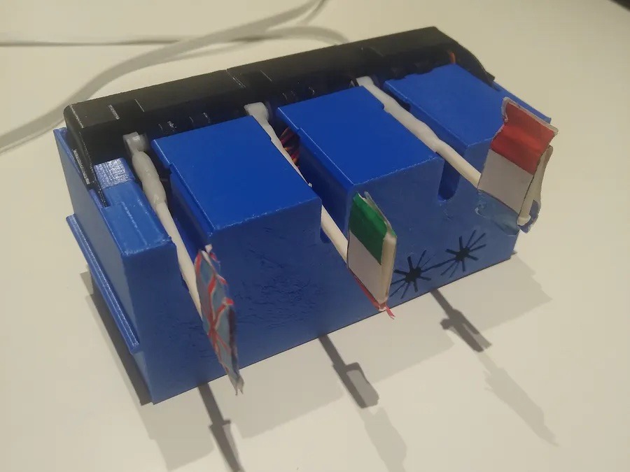
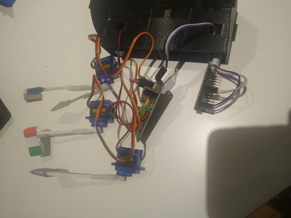
Although smartphone users have had the ability to quickly translate spoken words into nearly any modern language for years now, this feat has been quite tough to accomplish on small, memory-constrained microcontrollers. In response to this challenge, Hackster.io user Enzo decided to create a proof-of-concept project that demonstrated how an embedded device can determine the language currently being spoken without the need for an Internet connection.
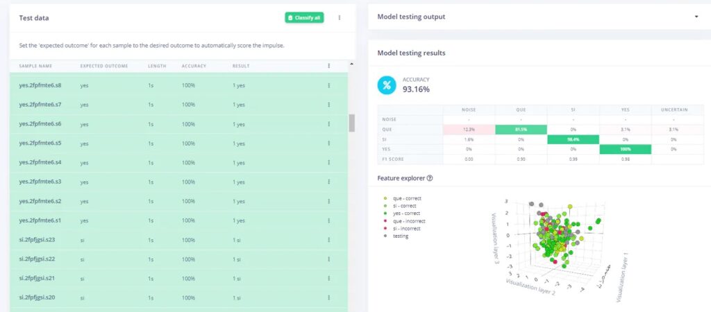
This so-called “language detector” is based on an Arduino Nano 33 BLE Sense, which is connected to a common PCA9685 motor driver that is, in turn, attached to a set of three micro servo motors — all powered by a single 9V battery. Enzo created a dataset by recording three words: “oui” (French), “si” (Italian), and “yes” (English) for around 10 minutes each for a total of 30 minutes of sound files. He also added three minutes of random background noise to help distinguish between the target keywords and non-important words.
Once a model had been trained using Edge Impulse, Enzo exported it back onto his Nano 33 BLE Sense and wrote a small bit of code that reads audio from the microphone, classifies it, and determines which word is being spoken. Based on the result, the corresponding nation’s flag is raised to indicate the language.
You can see the project in action below and read more about it here on Hackster.io.
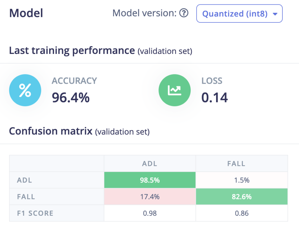
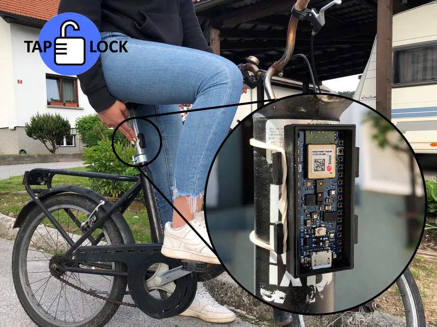
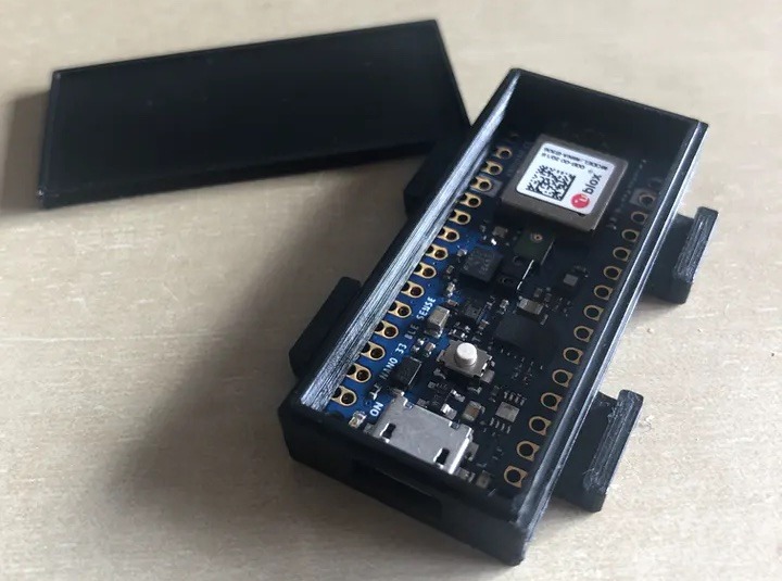
Bike locks have not changed that much in the last few decades, even though our devices have gotten far smarter, so they seem in need of an update. Designed with this in mind, the TapLock is able to intelligently lock and unlock from either Bluetooth or taps on the enclosure. It uses a Nano 33 BLE Sense to detect tap patterns via an onboard accelerometer as well as BLE capabilities to communicate with the owner’s phone.
Because taps are not necessarily directional, the TapLock’s creators took an average of each accelerometer axis and charted the time between the peaks. After collecting a large sample of data, they used Edge Impulse to process the data and then train a model with an accuracy of 96.4%. This allows the owner to have some wiggle room when trying to lock or unlock the bike.
The team also developed a mobile app, which provides another way for the bike’s owner to lock or unlock the bike, along with some extra features too. After connecting to the TapLock, the app loads the previous state of the lock device and updates itself if needed. If the user wants to lock the bike, the app will send a “lock” command to the TapLock and store the current location to show on a map. This way the owner won’t forget where their bike is when trying to retrieve it.
Currently, the TapLock doesn’t have a physical locking mechanism, but the team states that one can be added and then electronically activated from one of the Nano 33 BLE Sense’s GPIO pins. You can see a demo of this project in the video below and read about it on Hackster.io.
In this deep dive article, performance optimization specialist Larry Bank (a.k.a The Performance Whisperer) takes a look at the work he did for the Arduino team on the latest version of the Arduino_OV767x library.
Arduino recently announced an update to the Arduino_OV767x camera library that makes it possible to run machine vision using TensorFlow Lite Micro on your Arduino Nano 33 BLE board.
If you just want to try this and run machine learning on Arduino, you can skip to the project tutorial.
The rest of this article is going to look at some of the lower level optimization work that made this all possible. There are higher performance industrial-targeted options like the Arduino Portenta available for machine vision, but the Arduino Nano 33 BLE has sufficient performance with TensorFlow Lite Micro support ready in the Arduino IDE. Combined with an OV767x module makes a low-cost machine vision solution for lower frame-rate applications like the person detection example in TensorFlow Lite Micro.
Need for speed
Recent optimizations done by Google and Arm to the CMSIS-NN library also improved the TensorFlow Lite Micro inference speed by over 16x, and as a consequence bringing down inference time from 19 seconds to just 1.2 seconds on the Arduino Nano 33 BLE boards. By selecting the person_detection example in the Arduino_TensorFlowLite library, you are automatically including CMSIS-NN underneath and benefitting from these optimizations. The only difference you should see is that it runs a lot faster!
The CMSIS-NN library provides optimized neural network kernel implementations for all Arm’s Cortex-M processors, ranging from Cortex-M0 to Cortex-M55. The library utilizes the processor’s capabilities, such as DSP and M-Profile Vector (MVE) extensions, to enable the best possible performance.
The Arduino Nano 33 BLE board is powered by Arm Cortex-M4, which supports DSP extensions. That will enable the optimized kernels to perform multiple operations in one cycle using SIMD (Single Instruction Multiple Data) instructions. Another optimization technique used by the CMSIS-NN library is loop unrolling. These techniques combined will give us the following example where the SIMD instruction, SMLAD (Signed Multiply with Addition), is used together with loop unrolling to perform a matrix multiplication y=a*b, where
a=[1,2]
and
  b=[3,5
     4,6]
a, b are 8-bit values and y is a 32-bit value. With regular C, the code would look something like this:
However, using loop unrolling and SIMD instructions, the loop will end up looking like this:
a_operand = a[0] | a[1] << 16 // put a[0], a[1] into one variable
  for(i=0; i<2; ++i)
    b_operand = b[0][i] | b[1][i] << 16 // vice versa for b
    y[i] = __SMLAD(a_operand, b_operand, y[i])
This code will save cycles due to
fewer for-loop checks
__SMLAD performs two multiply and accumulate in one cycle
This is a simplified example of how two of the CMSIS-NN optimization techniques are used.
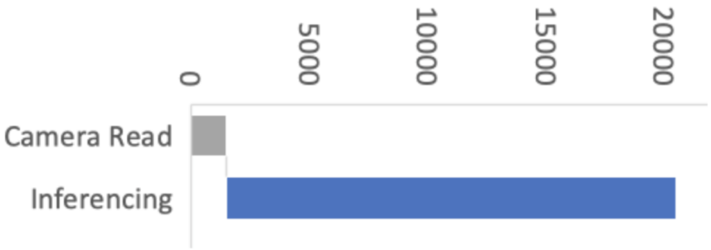
Figure 1: Performance with initial versions of libraries
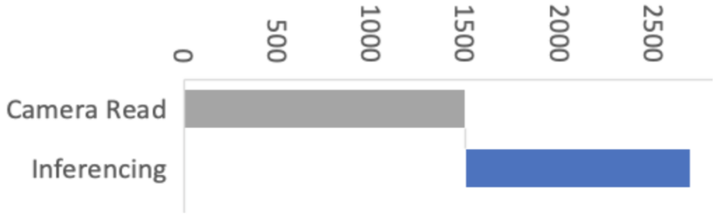
Figure 2: Performance with CMSIS-NN optimizations
This improvement means the image acquisition and preprocessing stages now have a proportionally bigger impact on machine vision performance. So in Arduino our objective was to improve the overall performance of machine vision inferencing on Arduino Nano BLE sense by optimizing the Arduino_OV767X library while maintaining the same library API, usability and stability.
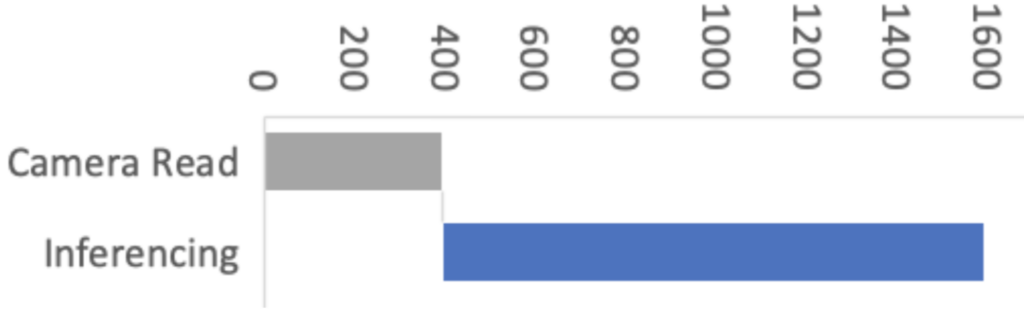
Figure 3: Performance with CMSIS-NN and camera library optimizations
For this, we enlisted the help of Larry Bank who specializes in embedded software optimization. Larry’s work got the camera image read down from 1500ms to just 393ms for a QCIF (176×144 pixel) image. This was a great improvement!
Let’s have a look at how Larry approached the camera library optimization and how some of these techniques can apply to your Arduino code in general.
Performance optimizing Arduino code
It’s rarely practical or necessary to optimize every line of code you write. In fact there are very good reasons to prioritize readable, maintainable code. Being readable and optimized don’t necessarily have to be mutually exclusive. However, embedded systems have constrained resources, and when applications demand more performance, some trade-offs might have to be made. Sometimes it is necessary to restructure algorithms, pay attention to compiler behavior, or even analyze timing of machine code instructions in order to squeeze the most out of a microcontroller. In some cases this can make the code less readable — but the beauty of an Arduino library is that this can be abstracted (hidden) from user sketch code beneath the cleaner library function APIs.
What does “Camera.readFrame” do?
We’ve connected a camera to the Arduino. The Arduino_OV767X library sets up the camera and lets us transfer the raw image data from the camera into the Arduino Nano BLE memory. The smallest resolution setting, QCIF, is 176 x 144 pixels. Each pixel is encoded in 2 bytes. We therefore need to transfer at least 50688 bytes (176 x 144 x 2 ) every time we capture an image with Camera.readFrame. Because the function is performing a byte read operation over 50 thousand times per frame, the way it’s implemented has a big impact on performance. So let’s have a look at how we can most efficiently connect the camera to the Arduino and read a byte of data from it.
Philosophy
I tend to see the world of code through the “lens” of optimization. I’m not advocating for everyone to share my obsession with optimization. However, when it does become necessary, it’s helpful to understand details of the target hardware and CPU. What I often encounter with my clients is that their code implements their algorithm neatly and is very readable, but it’s not necessarily ‘performance friendly’ to the target machine. I assume this is because most people see code from a top-down approach: they think in terms of the abstract math and how to process the data. My history in working with very humble machines and later turning that into a career has flipped that narrative on its head. I see software from the bottom up: I think about how the memory, I/O and CPU registers interact to move and process the data used by the algorithm. It’s often possible to make dramatic improvements to the code execution speed without losing any of its readability. When your readable/maintainable solution still isn’t fast enough, the next phase is what I call ‘uglification.’ This involves writing code that takes advantage of specific features of the CPU and is nearly always more difficult to follow (at least at first glance!).
Optimization methodology
Optimization is an iterative process. I usually work in this order:
Test assumptions in the algorithm (sometimes requires tracing the data)
Make innocuous changes in the logic to better suit the CPU (e.g. change modulus to logical AND)
Flatten the hierarchy or simplify overly nested classes/structures
Test any slow/fast paths (aka statistics of the data — e.g. is 99% of the incoming data 0?)
Go back to the author(s) and challenge their decisions on data precision / storage
Make the code more suitable for the target architecture (e.g. 32 vs 64-bit CPU registers)
If necessary (and permitted by the client) use intrinsics or other CPU-specific features
Go back and test every assumption again
If you would like to investigate this topic further, I’ve written a more detailed presentation on Writing Performant C++ code.
Depending on the size of the project, sometimes it’s hard to know where to start if there are too many moving parts. If a profiler is available, it can help narrow the search for the “hot spots” or functions which are taking the majority of the time to do their work. If no profiler is available, then I’ll usually use a time function like micros() to read the current tick counter to measure execution speed in different parts of the code. Here is an example of measuring absolute execution time on Arduino:
long lTime;
  lTime = micros();
  <do the work>
  iTime = micros() - lTime;
  Serial.printf(“Time to execute xxx = %d microseconds\n”, (int)lTime);
I’ve also used a profiler for my optimization work with OpenMV. I modified the embedded C code to run as a MacOS command line app to make use of the excellent XCode Instruments profiler. When doing that, it’s important to understand how differently code executes on a PC versus embedded — this is mostly due to the speed of the CPU compared to the speed of memory.
Pins, GPIO and PORTs
One of the most powerful features of the Arduino platform is that it presents a consistent API to the programmer for accessing hardware and software features that, in reality, can vary greatly across different target architectures. For example, the features found in common on most embedded devices like GPIO pins, I2C, SPI, FLASH, EEPROM, RAM, etc. have many diverse implementations and require very different code to initialize and access them.
Let’s look at the first in our list, GPIO (General Purpose Input/Output pins). On the original Arduino Uno (AVR MCU), the GPIO lines are arranged in groups of 8 bits per “PORT” (it’s an 8-bit CPU after all) and each port has a data direction register (determines if it’s configured for input or output), a read register and a write register. The newer Arduino boards are all built around various Arm Cortex-M microcontrollers. These MCUs have GPIO pins arranged into groups of 32-bits per “PORT” (hmm – it’s a 32-bit CPU, I wonder if that’s the reason). They have a similar set of control mechanisms, but add a twist — they include registers to SET or CLR specific bits without disturbing the other bits of the port (e.g. port->CLR = 1; will clear GPIO bit 0 of that port). From the programmer’s view, Arduino presents a consistent set of functions to access these pins on these diverse platforms (clickable links below to the function definitions on Arduino.cc):
For me, this is the most powerful idea of Arduino. I can build and deploy my code to an AVR, a Cortex-M, ESP8266 or an ESP32 and not have to change a single line of code nor maintain multiple build scripts. In fact, in my daily work (both hobby and professional), I’m constantly testing my code on those 4 platforms. For example, my LCD/OLED display library (OneBitDisplay) can control various monochrome LCD and OLED displays and the same code runs on all Arduino boards and can even be built on Linux.
One downside to having these ‘wrapper’ functions hide the details of the underlying implementation is that performance can suffer. For most projects it’s not an issue, but when you need to get every ounce of speed out of your code, it can make a huge difference.
Camera data capture
One of the biggest challenges of this project was that the original OV7670 library was only able to run at less than 1 frame per second (FPS) when talking to the Nano 33. The reason for the low data rate is that the Nano 33 doesn’t expose any hardware which can directly capture the parallel image data, so it must be done ‘manually’ by testing the sync signals and reading the data bits through GPIO pins (e.g. digitalRead) using software loops. The Arduino pin functions (digitalRead, digitalWrite) actually contain a lot of code which checks that the pin number is valid, uses a lookup table to convert the pin number to the I/O port address and bit value and may even disable interrupts before reading or changing the pin state. If we were to use the digitalRead function for an application like this, it would limit the data capture rate to be too slow to operate the camera. You’ll see this further down when we examine the actual code used to capture the data.
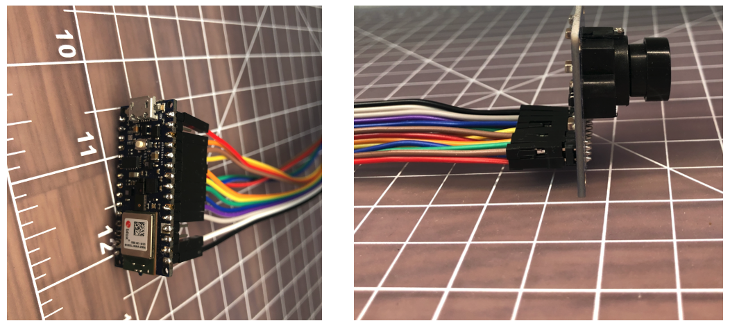
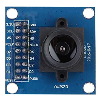
First, a quick review of the OV7670 camera module: According to its datasheet, it’s capable of capturing a VGA (640×480) color image at up to 30 FPS. The kit used for this project has the camera mounted to a small PCB and presents an 8-bit parallel data bus and various sync signals.
It requires an external “master clock” (MCLK in the photo) to drive its internal state machine which is used to generate all of the other timing signals. The Nano 33 can provide this external clock source by using its I2S clock. The OV767X library sets this master clock to 16Mhz (the camera can handle up to 48Mhz) and then there is a set of configuration registers to divide this value to arrive at the desired frame rate. Only a few possible frame rates are available (1, 5, 10, 15, 20, and 30 FPS).
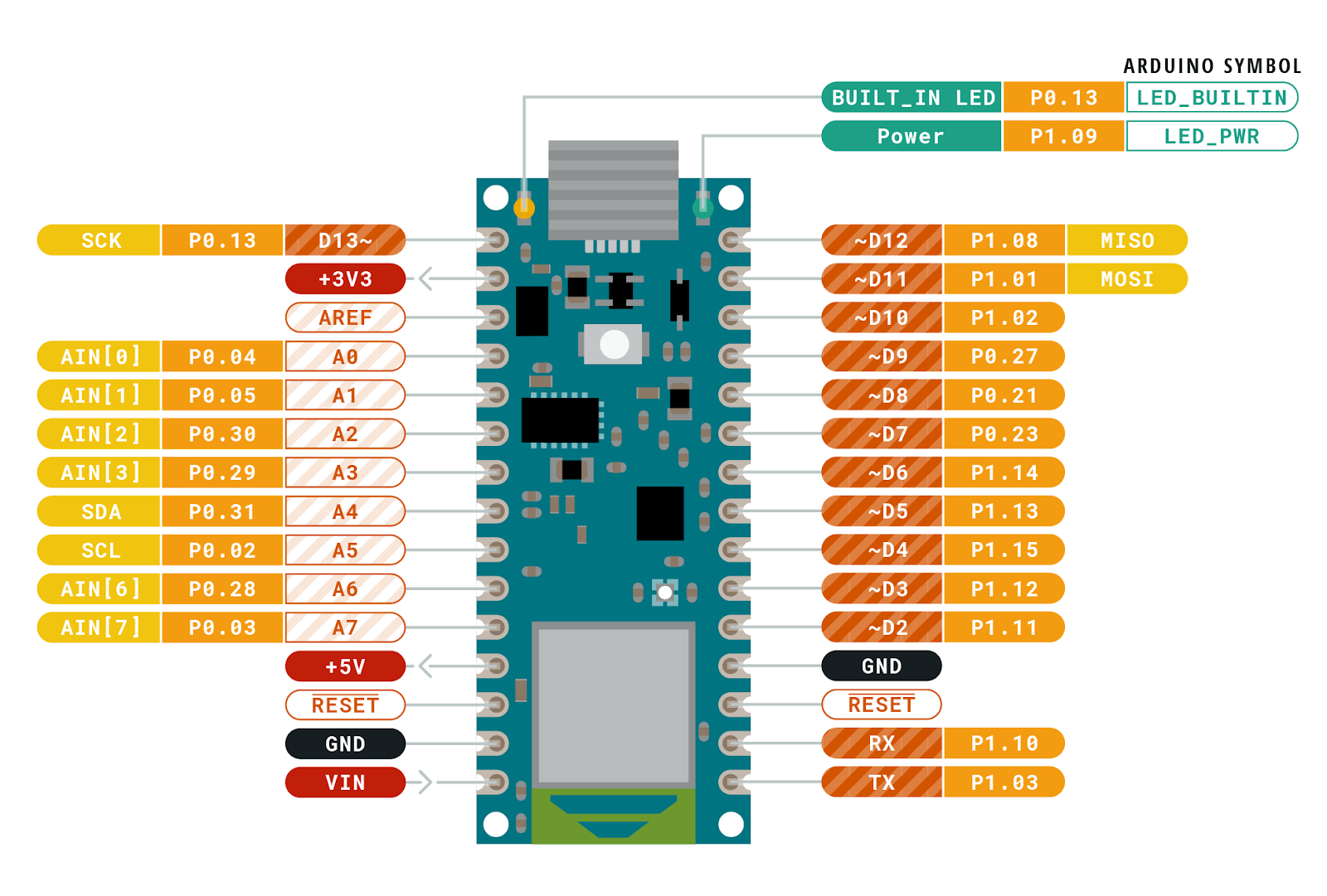
Above is one of the timing diagrams from the OV7670 datasheet. This particular drawing shows the timing of the data for each byte received along each image row. The HREF signal is used to signal the start and end of a row and then each byte is clocked in with the PCLK signal. The original library code read each bit (D0-D7) in a loop and combined them together to form each data byte. The image data comes quickly, so we have very little time to read each byte. Assembling them one bit at a time is not very efficient. You might be thinking that it’s not that hard of a problem to solve on the Nano 33. After all, it has 22 GPIO pins and the Cortex-M inside it has 32-bit wide GPIO ports, so just hook up the data bits sequentially and you’ll be able to read the 8 data bits in one shot, then Mission Accomplished. If only things were that easy. The Nano 33 does have plenty of GPIO pins, but there isn’t a continuous sequence of 8 bits available using any of the pins! I’m guessing that the original code did it one bit at a time because it didn’t look like there was a better alternative. In the pinout diagram below, please notice the P0.xx and P1.xx numbers. These are the Cortex-M GPIO port 0 and 1-bit numbers (other Cortex-M processors would label them PA and PB).
I wasn’t going to let this little bump in the road stop me from making use of bit parallelism. If you look carefully at the bit positions, the best continuous run we can get is 6 bits in a row with P1.10 through P1.15. It’s not possible to read the 8 data bits in one shot…or is it? If we connect D0/D1 of the camera to P1.02/P1.03 and D2-D7 to P1.10-P1.15, we can do a single 32-bit read from port P1 and get all 8 bits in one shot. The bits are in order, but will have a gap between D1 and D2 (P1.04 to P1.09). Luckily the Arm CPU has what’s called a barrel shifter. It also has a smart instruction set which allows data to be shifted ‘for free’ at the same time the instruction is doing something else. Let’s take a look at how and why I changed the code:
Original:
uint8_t in = 0;
  for (int k = 0; k < 8; k++) {
     bitWrite(in, k, (*_dataPorts[k] & _dataMasks[k]) != 0);
  }
Optimized:
  uint32_t in = port->IN; // read all bits in parallel
  in >>= 2; // place bits 0 and 1 at the "bottom" of the
register
  in &= 0x3f03; // isolate the 8 bits we care about
  in |= (in >> 6); // combine the upper 6 and lower 2 bits
Code analysis
If you’re not interested in the nitty gritty details of the code changes I made, you can skip this section and go right to the results below.First, let’s look at what the original code did. When I first looked at it, I didn’t recognize bitWrite; apparently it’s not a well known Arduino bit manipulation macro; it’s defined as:
This macro was written with the intention of being used on GPIO ports (the variable value) where the logical state of bitvalue would be turned into a single write of a 0 or 1 to the appropriate bit. It makes less sense to be used on a regular variable because it inserts a branch to switch between the two possible outcomes. For the task at hand, it’s not necessary to use bitClear() on the in variable since it’s already initialized to 0 before the start of each byte loop. A better choice would be:
if (*_dataPorts[k] & _dataMasks[k]) in |= (1 << k);
The arrays _dataPorts[] and _dataMasks[] contain the memory mapped GPIO port addresses and bit masks to directly access the GPIO pins (bypassing digitalRead). So here’s a play-by-play of what the original code was doing:
Set in to 0
Set k to 0
Read the address of the GPIO port from _dataPorts[] at index k
Read the bit mask of the GPIO port from _dataMasks[] at index k
Read 32-bit data from the GPIO port address
Logical AND the data with the mask
Shift 1 left by k bits to prepare for bitClear and bitSet
Compare the result of the AND to zero
Branch to bitSet() code if true or use bitClear() if false
bitClear or bitSet depending on the result
Increment loop variable k
Compare k to the constant value 8
Branch if less back to step 3
Repeat steps 3 through 13, 8 times
Store the byte in the data array (not shown above)
The new code does the following:
Read the 32-bit data from the GPIO port address
Shift it right by 2 bits
Logical AND (mask) the 8 bits we’re interested in
Shift and OR the results to form 8 continuous bits
Store the byte in the data array (not shown above)
Each of the steps listed above basically translates into a single Arm instruction. If we assume that each instruction takes roughly the same amount of time to execute (mostly true on Cortex-M), then old vs. new is 91 versus 5 instructions to capture each byte of camera data, an 18x improvement! If we’re capturing a QVGA frame (320x240x2 = 153600 bytes), that becomes manymillionsof extra instructions.
Results
The optimized byte capture code translates into 5 Arm instructions and allows the capture loop to now handle a setting of 5 FPS instead of 1 FPS. The FPS numbers don’t seem to be exact, but the original capture time (QVGA @ 1 FPS) was 1.5 seconds while the new capture time when set to 5 FPS is 0.393 seconds. I tested 10 FPS, but readFrame() doesn’t read the data correctly at that speed. I don’t have an oscilloscope handy to probe the signals to see why it’s failing. The code may be fast enough now (I think it is), but the sync signals may become too unstable at that speed. I’ll leave this as an exercise to the readers who have the equipment to see what happens to the signals at 10 FPS.
For the work I did on the OV767X library, I created a test fixture to make sure that the camera data was being received correctly. For ML/data processing applications, it’s not necessary to do this. The built-in camera test pattern can be used to confirm the integrity of the data by using a CRC32.
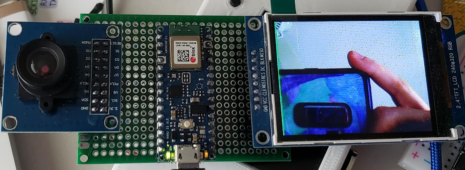
My tinned protoboard test fixture with 320×240 LCD
Note: The frames come one immediately after another. If you capture a frame and then do some processing and then try to capture another frame, you may hit the middle of the next frame when you call readFrame(). The code will then wait until the next VSync signal, so that frame’s capture time could be as much as 2x as long as a single frame time.
More tips
I enjoy testing the limits of embedded hardware, especially when it involves bits, bytes and pixels. I’ve written a few blog posts that explore the topics of speed and power usage if you’re interested in learning more about it.
Conclusion
The embedded microcontrollers available today are capable of handling jobs that were unimaginable just a few years ago.
Optimized ML solutions from Google and Edge Impulse are capable of running on low-cost, battery-powered boards (vision, vibration, audio, whatever sensor you want to monitor).
Python and Arduino programming environments can test your project idea with little effort.
Software can be written an infinite number of ways to accomplish the same task, but one constant remains: TANSTATFC (there ain’t no such thing as the fastest code).
Never assume the performance you’re seeing is what you’re stuck with. Think of existing libraries and generic APIs available through open source libraries and environments as a starting point.
Knowing a bit of info about the target platform can be helpful, but it’s not necessary to read the MCU datasheet. In the code above, the larger concept of Arm Cortex-M 32-bit GPIO ports was sufficient to accomplish the task without knowing the specifics of the nRF52’s I/O hardware.
Don’t be afraid to dig a little deeper and test every assumption.
If you encounter difficulties, the community is large and there are a ton of resources out there. Asking for help is a sign of strength, not weakness.
About
Planet Arduino is, or at the moment is wishing to become, an aggregation of public weblogs from around the world written by people who develop, play, think on Arduino platform and his son. The opinions expressed in those weblogs and hence this aggregation are those of the original authors. Entries on this page are owned by their authors. We do not edit, endorse or vouch for the contents of individual posts. For more information about Arduino please visit www.arduino.cc
You are currently browsing the archives for the Tiny Machine Learning category.


 . If only things were that easy. The Nano 33 does have plenty of GPIO pins, but there isn’t a continuous sequence of 8 bits available using any of the pins! I’m guessing that the original code did it one bit at a time because it didn’t look like there was a better alternative. In the pinout diagram below, please notice the P0.xx and P1.xx numbers. These are the Cortex-M GPIO port 0 and 1-bit numbers (other Cortex-M processors would label them PA and PB).